whore Л/, i is the marginal rale of substitution between dates I and 7, and 5 is the rate of time preference. Ibis welt-known equilibrium asset-pricing relation equates current price of the security to its expected discounted ftiturt- payoff, discounted using the stochastic discount factor.

Lucas (1078) observes that (12.3.25) need not imply a martingale process for (/ supporting l.eroys (1973) contention that the martingale properly is neither a necessary nor sufficient condition for rationally determined asscl prices. However, assuming that the conditional distribution of future consumption has a density representation /( ), the conditional expectation in (12.3.25) can be re-expressed in the following way:

F., Y(CT)M,.r\ = f Y((:,)- lr) MCr)dC, (I2.3.2C.)

= г---7 J Y(CT)/.(С,) dC, (12.3.2

whore

F.;)(C-V)]. (12.3.28)

/,((.,) = ~.- -, (12.3.2))

J Л/,.rj, :-i )dCr

and i, у is ihe continuously compounded net rate of return between / and 7 of an asset promising one unit of consumption at 7; i.e., it is the return on the riskless asset.

This version of the F.uler equation shows dial an assets current price can be expressed as ils discounted expected payoff, discounted at the riskless rale of interest (see Chapter 8 for a more detailed discussion). However, the expectation is taken with respect lo (he.SPD/*, a marginal-rate-of-substitution-wcighied probability density function, not the original probability density (unction / of future consumption. In a continuous-time selling, /* is also known as ihe risk-neutral pricing density (Cox and Ross [1976]) or the ei/uiv-alenl martingale measure (Harrison and Krcps [ 107.)]).ir

Once j is obtained, it cm be used lo price any asset at dale t with a single liquidating payoff at date 7 that is an arbitrary function of consumption (./. SPDs also provide the link belween preference-based equilibrium models of the type discussed in Chapter 8 and arbitrage-based derivative pricing models of die type discussed in Chapter 9. Indeed, implicit in the

Sec I lii.nit; .niil l.ii/cnhcigci (I.IHK. (:haptcr fi) lor a more detailed discussion ol.SIOs.

Sei uriiies wiili multiple >.ivolls and inliuiie horizons can also he priced try (he SIM), hut in these cases the SII) must he appropriately redefined lo capture ihe time-variation in the marginal tales of substitution-see llrccdcn and t.ii/enhcrger ( H>7k) and Radner (I.Wi) lot further discussion.

ПС) 1 + exp[-/6(C-a)] +Ь

a > 0, b < 0 (12.3.32)

a s c+!og(-a/i). (12.3.33)

This payoff function is a smoothed version of the payoff to an option portfolio commonly known as bullish vertical spread, in which a call option with a low strike is purchased and a call option with a high strike price is written (see Figure 12.5 and Cox and Rubinstein [1985, Chapter 1] for further details).

Extracting SPDs from Derivatives Prices There is an even closer relation between option prices and SPDs than (12.3.30) suggests, which Ross (1976), Banzand Miller (1978), and Breeden and Lilzenberger (1978) first discovered. In particular, they show that the second derivative of the call-pricing function G, with respect to the strike

prices of all financial securities-derivatives or not-are the prices of Anpw- v,., Debrett securities, and these prices may be used to value all other securities, :, no matter how complex.

Pricing Derivatives with SPDs

Under some regularity conditions, we may express f as an explicit function of / and 7 so that a single SPD /*(СГ; (, T) may be used to price an asset at any date / with a single liquidating payoff Y{CT) at any future date T > t (see footnote 16):

p, = e-..HT-n j Y(CT)f(Cr; t, T)dCT, (12.3.30)

and we shall adopt this convention for notational simplicity. For example, a European call option on date-/ aggregate consumption CT with strike price X has a payoff function Y{CT) = max[CT - X, 0] and hence its date-i price G, is simply

G, = r- ,T- JmaxtC - X,0}f(Cnt,T)dCT. (12.3.31)

Even the most complex path-independent derivative security can be priced and hedged according to (12.3.30). For example, consider a security with the highly nonlinear payoff function:

X Ш Ш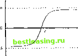

Figure 12.6. Ilullish Vertical Spreiul Payoff Function and Smoothed Vers,

price X must equal the SPD:

..r(/-

(12.3.34)

Therefore, impounded in every option pricing formula is the SPD /*. To estimate the SPD using (12.3.34), we require a call option pricing formula. Although many parametric pricing formulas exist (see 1 lull [1993, Chapter 17] for some popular examples), Att-Sahalia and l .о (1990) construct a nonparamelric pricing formula that places fewer restrictions- pjrimarily smoothness and weak dependence-on the data-generating process of the underlying assets price. While parametric formulas such as djiose of Black and Scholes (1973) and Merlon (1973) offer great advantages when the parametric assumptions (e.g., geometric Brownian motion) a-e satisfied, nonparametric methods arc robust to violations оГ these as-si imptions. Since there is some empirical evidence that casts doubt on such assumptions, at least for stock indexes,17 the nonparametric approach may have some important advantages. 1

Given observed call option prices (G X/, r,j (vdrcre r, s ]) - I,), the prices of the underlying asset \P,\, and the riskless rate of interest rrJ, we may construct the smooth nonparametric call-pricing functibn as

G(P,X, r, rr) = E[G I P, X, r, rx]

(12.3.35)

using a multivariate kernel A., formed as a product of </=4 univariate kernels: W,X,r,r,) = A*>(/)ft ,(X)AAl(r)A*,(rr). (12.3.30)

Secl-d and MacKinlay (1УНН), lor example.

See Hutchinson, I-o, and Poggio (1994) and Ait-Sahalia (I9.)6a) for oilier nonparatneti ir oplion pricing alternatives.

and hence

G(l> X г г ) = w-MX ~ Y->Mr ~ r.>M ~ r )C,

E!Li ht(P-Л)*/ (X - X,)A r(r - r,)A ,(rr - rr)

(12.3.37)

The options delta and SIT) estimator then follow by dilleienliating /:

Д(ЛХ,г,гт) = I (12.3.38)

fiP-r I Я,г,гг) =

<)( ;(/, x, r ,) ax*

. (12.3.39)

x=/7

Under standard regularity assumptions on the data-generating process as well as smoothness assumptions on the true call-pricing function, Ait-Sabalia and l.o (1990) show that the estimators of the option price, the options delta, and the SPD are all consistent and asymptotically normal, and they provide explicit expressions for the asymptotic variances.

Armed with the SPD, any derivative security with characteristic < and payoff function K(f, 1,) al T=l + r can now be priced at date (by the pricing function:

/ OO

GU.f.r, ;>) = ,ГГ / Y(r,Pr)f(Pr I p,r,r,)dPr. (12.3.40) Jo

If the payoff function Y(-) is twice-diflereiuiable in /,-, then

/ no

G(I\r, r, rr) = Trr / Y(r,Pr) /*( I P,T.r,)dP, (12.3.41) Jo

f°° , dlG

= / УЦ,Рт)-rrdlr (12.3.42) Jo д Pj-

r°° а2У(с, /V) -

= l -Щ-СНРг. (12.3.43)

Integrating against G instead of its second derivative speeds up the convergence rate of the estimator-G converges at speed ni/2 пл,г and its integral against a smooth function of Ir converges al speed 1сл/г, whereas the second derivative of G converges at n1 hH/~ and its integral against a smooth function of PT at n12 h/2. A factor of lvi/2 is gained in the speed of convergence by integrating the second derivative of the payoff function-when it exists-against G instead of integrating the payoff function itself against the second derivative of G.

I/. Nonlinearities in Financial Data

Ait-Sahalia and l.o (1!)%) apply I his estimator lo die pricing and delta-hedging ol S.4.T 500 call and ptii options using daily daia obtained from the Chicago Board Options Exchange lor the sample period from January I, 1993 to December .41, 1993, yielding a total sample size of 14,431 observations. The estimates of the SlDs exhihit negative skewness and excess kuriosis, a common feature of historical slock returns (see Chapter I for example). Also, unlike many parametric option pricing models, the SPD-geuerated option pricing formula is capable ofeapturing persistent volatility smiles and other empirical features of market prices.

12.4 Artificial Neural Networks

An alternative to noiiparameti ic regression that has received much recent attention in the engineering and business communities is the artificial neural network. Artificial neural networks may he viewed as a nonparamelric let h-ni(iie, heme these models would lit rtiite naturally in Section 12.3. 1 low-ever, because initially thevdrew their motivation from biological phenomena-in particular, from the physiology of nerve cells-they have become pari of a separate, distinct, and burgeoning literature (see Hertz, Krogh, and Palmer IM.) I , 11 it к binson, I .<>, and Poggio 1994 ], Poggio and Cirosi [ 1990, and White J I992 for overviews of this literature).

To underscore the common nonparametric origins of artificial neural networks, we describe three kinds of networks in this section, collectively known as learning networks (see Barron and Barron [1988]). In Section 12.4.1 we introduce the multilayer perceptron, perhaps the most popular type of artificial neural network in the recent literature-this is what the term neural network is usually taken to mean. In Sections 12.4.2 and 12.4.3 we present two other techniques dial also have network interpretations: radial basis functions, and projection pursuit regression.

12. 1.1 Multilayer Ierreptrons

Perhaps the simplest example of an artificial neural network is the binary threshold inailel of McCulloch and Pills (1913), in which an output variable > taking on only ihe values zero and one is noiilinearly related lo a collection of / input variables Sr j - I...../ in the following way:

r = (i(l>A-i<) dii.t)

12.4. Artificial Neural Nettvorks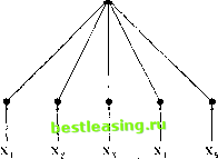

Input Layer

Figure 12.7. Binary Threshold Model

According to (12.4.1), each input Xj is weighted by a coefficient /3;, called the connection strength, and then summed across all inputs. If this weighted sum exceeds the threshold fj., then the artificial neuron is switched on or activated via the activation function g(-); otherwise it remains dormant. This simple network is often represented graphically as in Figure 12.7, in which the input layer is said to be connected to the output layer.

Generalizations of the binary threshold model form the basis of most current applications of artificial neural network models. In particular, to allow for continuous-valued outputs, the Heaviside activation function (12.4.2) is replaced by the logistic function (see Figure 12.8):

£(u) = T+h~ - {12A3)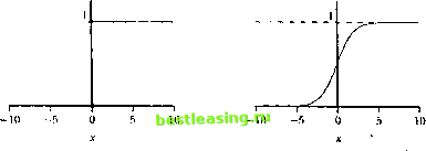

Figure 12.8. Comparison of Heaviside and logistic Activation Functions