ЧИР

г

/2. Nonlinearilies in Financial Data

Output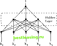

Input ltycr

Figure 12.9. Multilayer lercefitmn with a Single Hidden Layer

Also, without loss of generality, we set pi to zero since il is always possible to model a nonzero activation level by defining the first input X = l in which case the negative of that inputs connection strength -fi\ becomes the activation level.

But perhaps the most important extension of the binary threshold model is the introduction of a hidden layer between the input layer and the output layer. Specifically, let

Y = A(£atg(3;X)J (12.4.4)

Pk = [Ai Pa Pkj ], X = [X,

where h(-) is another arbitrary nonlinear activation function. Willis case, the inputs arc connected to multiple hidden units, and at each hidden unit they are weighted (differently) and transformed by the (same) activation function g(-). The output of each hidden unit is then weighted ycyigaiu- this time by the a s-and summed and transformed bya second activation function Л(). Such a network configuration is an example of a multilayer perceplron (MI.P)-a single (hidden) layer in this case-and is perhaps the mosl common type of artificial neural network among recent applications. In contrast to Figure 12.7, the multilayer pcrceptron has a more complex network topology (see Figure 12.9). This can be generalized in the obvious . way by adding more hidden layers, hence the term multilayer perceplron.

For a given set of inputs and outputs X Y,}, MI.P approximation amounts to estimating the parameters of the MI.P network-the vectors

(Зк and scalars a , fc=l.....К-typically by minimizing the sum of squared

deviations between the output and the network, i.e., £,[ Ii- - £itof*r.r(0*X)]2-

12.4. Artificial Neural Networks

In the terminology of this literature, the process of parameter estimation is called training Ihe network. This is less pretentious than il may appear to be-an early method of parameter estimation was backpmpagalion, and this does mimic a kind of learning behavior (albeit a very simplistic one).19 However, While (1992) cites a number of practical disadvantages with backprop-agation (numerical instabilities, occasional non-convergence, etc.), hence the preferred method for estimating the parameters of (12.4.4) is nonlinear least-squares.

F.vcn the single hidden-layer MI.P (12.4.4) possesses the universal ajr-proximation property: It can approximate any nonlinear function lo an arbitrary degree of accuracy with a suitable number of hidden units (sec White [ 1992]). However, the universal approximation property is shared by many nonparametric estimation techniques, including the nonparametric regression estimator of Section 12.3, and the techniques in Sections 12.4.2 and 12.4.3. Of course, this tells us nothing about the performance of such techniques in practice, and for a given set of data it is possible for one technique to dominate another in accuracy and in other ways.

Perhaps the mosl important advantage of MLPs is their ability lo approximate complex nonlinear relations through the composition of a network of relatively simple functions. This specification lends itself naturally to parallel processing, and although there are currently no financial applications that exploit this feature of MLPs, this may soon change as parallel-processing software and hardware become more widely available.

To illustrate the MLP model, we apply il to the artificial dataset generated by (12.3.1 1). For a network with one hidden layer and live hidden units, denoted by MLP(1,5), with (-)() set to the identity function, we obtain the following model:

) , = 5.282 - 14.576g(-1.472 + 1.809 X,)

- 5.4 llg(-2.628 4-0.04 IX,)

- 3.071(13.288 - 2.347X,) + (i.320g(-2.009 4- 4.009X,)

+ 7.892g(-3.316 + 2.484X,) (12.4.5)

where g(u) = 1/(1 -f e~ ). This model is plotted in Figure 12.10 and compares well with the kernel estimator described in Section 12.3.1. Dcspilc the fact thai (12.4.5) looks nothing like die sine function, nevertheless die MLP performs quite well numerically and is relatively easy to estimate.

-backpropagation is essentially lite method ol \Uicha\lir tipjmixnniilmti tits! proposed by Robbins and Monro (lilSIa). See While (IIMI2) lot Tin thet details.

i . ,\oiitineaiUies in /inauciat Ualii

Figure 12.10. ,\U.I(/.5) ЛЫс/of У, = Sin(X,) + О.Гк,

/2.7.2 Hiidinl linsis Functions

Till class dl initial husis junctions (RBEs) were first used to solve interpolation problems-fitting a curve exactly through a set of points (see Powcl! [ 1987] for a review). More recently, RBEs have been extended by several researchers to perforin the more general task of approximation (see Broomhead and Lowe I I988, Moody and Darken 19891,and Poggio and Girosi 11990]). In particular, Poggio and Girosi (199(1) show how RBFscan he derived from the classical rrgnlariiation problem in which some unknown function Г=ш(Х) is to be approximated given a sparse datasel (X/, У,) and some smoothness constraints. In terms of our multiple-regression antilogy, the (/-dimensional vector X/ are the explanatory variables, Y, the dependent variable, and m(-) the possibly nonlinear function lhat is the conditional expectation of ), given X and heme

Y, = i,i(X,) t f Ee,X, = 0. (12.4.0)

The i egulai i/.tlion (or nonparamelric estimation) problem may then be viewed as the iniiiiiiii/alion of die following objective functional:

Vim) ~ ( >/ - iii{X,)f + A.P/ (X,)-) . (12.-1.7)

12.-I. Artificial Neural Networks

where j is some vector norm and V is a differential operator. The firii term of the sum in (12.4.7) is simply the distance between m(X,) and the observation > the second term is a penalty function that is a decreasing* function of the smoothness of ( ), and X controls the tradeoff between smoothness and fit.

In its most general form, and under certain conditions (see, for example, Poggio and Girosi [1990]), the solution lo the minimization of (12.4.7) is given by the following expression:

m(X,) = Ам*(1Х(-и*)-гР(Х)-, (12.4.8)

where (U*J are rf-dimensional vector centers (similar to the knots of spline functions), {Bk) are scalar coefficients, [щ] are scalar functions, V(-) is a polynomial, and К is typically much less than the number of observations T in the sample. Such approximants have been termed hyperbasisfunctions by Poggio and Girosi (1990) and are closely related to splines, smoothers such as kernel estimators, and other nonparametric estimators.20

For our current purposes, we shall take the vector norm to be a weighted Euclidean norm defined by a {d x d) weighting-matrix W, and we shall take the polynomial term to be just the linear and constant terms, yielding the following specification for ( ):

m(X,) = a0 + a\X, + ]Г ДА ((X, - U*)WW(X, - U*)) , (124.9)

where от and ai are the coefficients of the polynomial V-). Miccheli (1)86) shows that a large class of basis functions жц(-) are appropriate, but the most common choices for basis functions are Gaussians e~*l and multiquadrics ч/л 4-02.

Networks of this type can generate any real-valued output, but in applications where we have some a priori knowledge of the range of the desired outputs, it is computationally more efficient to apply some nonlinear transfer function to the outputs to reflect lhat knowledge. This will be the case in our application to derivative pricing models, in which some of the RBF networks will be augmented with an output sigmoid, which maps the range (-oo, oo) into the fixed range (0, I). In particular, the augmented network will be of the form gin(x)) where g(u) = 1/(1 + e~ ).

As with MI.Ps, RBF approximation for a given set of inputs and outputs (X У,), involves estimating the parameters of the RBF network-the

- To economize on terminology, here we use RBKs lo encompass Ixilh the interpolation techniques used by Powell (1W7) and their subsequent generalizations.

d(d+1 )/2 unique entries of the matrix W W, the rt7< elements of ihe centers and the d+k+ 1 coefficients ото, oi, and (/)),)-typically hy nonlinear least-squares, i.e., by minimizing К/- я(Х,)]!! numerically.

12.4.3 Projection Pursuit Regression

Projection pursuit is a method that emerged from the statistics community for analyzing high-dimensional dalascts by looking al their low-dimensional projections. Friedman and Stuelzle (1981) developed a version for the nonlinear regression problem called projection pursuit regression (PPR). .Similar to MI.Ps, PPR models arc composed of projections of the data, i.e., products of the data with estimated coefficients, but unlike MI.Ps they also estimate the nonlinear combining functions from the data. Following the botation of Section 12.4.1, the formulation for PPR with a univariate output can be written as

m(X,) = exq 4- yatiffl),03),X,) *=t

(12.4.10)

where the functions m*(-) are estimated from the data (typically with a smoother), the (or*) and (/3*) are coefficients, К is the number of projections, and an is commonly taken to be the sample mean of the outputs m(X,). The similarities between PPR, RBF, and МЕР networks should be apparent from (12.4.10).

12.4.4 Limitations of Learning Networks

Despite the many advantages that learning networks possess for approximating nonlinear functions, they have several important limitations. In particular, there are currently no widely accepted procedures for4etermin-ing the network architecture in a given application, e.g., the number оГ hidden layers, the number of hidden units, the specification of the activation function(s), etc. Although some rules of thumb have emerged from

casual empirical observation, they are heuristic at best.

Difficulties also arise in training the network. Typically, network parameters arc obtained by minimizing the sum of squared errors, but because of the nonlinearities inherent in these specifications, the objective function 3 may not be globally convex and can have many local minima. JJiH. Finally, traditional techniques of statistical inference such as significance

в* testing cannot always be applied to network models because of the nesting of m layers. For example, if one of the arts in (12.4.4) is zero, then the connection

mr strengths (3k of that hidden unit are unidentified. Therefore, even simple

im. significance tests and confidence intervals require complex combinations ♦ of maintained hypotheses to be interpreted properly.

12.4.5 Application: I .earning the Hlaclt-Scholes Formula

(Vivcn the power and flexibility of neural networks lo approximate complex nonlinear relations, a natural application is to derivative securities whose pricing formulas are highly nonlinear even when they are available in closed form. In particular, Hutchinson, l.o, and Poggio (1994) pose the following challenge: If option prices were truly determined by the Black-Scholes formula exactly, can neural networks learn the Black-Scholes formula? In more standard statistical jargon: Can the Black-Scholes lot inula be estimated nonparamctrically via learning networks with a sufficient degree of accuracy to be of practical use?

Hutchinson, Lo, and Poggio (1994) lace this challenge by performing Monte Carlo simulation experiments in which various neural networks are trained on artificially generated Black-Scholes option prices and then compared to the Black-Scholes formula both analytically and in oul-of-sample hedging experiments to sec how close they come. Fven with training scLs of only six months of daily data, learning network pricing formulas can approximate the Black-Scholes formula with reasonable accuracy.

Specifically, they begin by simulating a two-year sample оГ daily stock prices, and creating a cross-section of options each day according to the rules used by the Chicago Board Options Exchange with prices given by the Black-Scholes formula. They refer to this two-year sample of stock and (multiple) option prices as a single trainingpalh, since the network is trained on this sample.21 Given a simulated training path (/(Ol of daily stock prices, they construct a corresponding path of option prices according to the rules of the Chicago Board Options Exchange (СВОЕ) for introducing options on stocks.

A typical training path is shown in Figure 12.11. Because the options generated for a particular sample path arc a function of the (random) stock price path, the size of this data matrix (in terms of number of options and total number of data points) varies across sample paths. For their training set, the number of options per sample path range from 71 to 91, with an average of 81. The total number of data points range (iom 5,227 to 6,847, with an average of 6,001.

The nonlinear models obtained from neural networks yield estimates

-They assume that ihe underlying asset for ihe simulation experiments is a typical NYSE stork, with an initial price /(()) of $50.00, an annual continuously compounded expected rale ol i el urn fi of 10%, and an annual volatility n ol 20%. tinder (he lilac k-S< holes assumption of a geometric brownian motion,

,11 = iilill + oliill.

and taking the number of days per year to be zTi.l, they draw TiOti pseudorandom variates ,) I tout tliedisiributionyV(/(/2.r):-l.a/25:t) to obtain two years of daily continuously compounded returns, which are converted lo prices with the usual relation /(() = ( >ехрГ] f, for (>0.