Optimal control theory has been important in finance (Islam and Craven [38, 2002]; Taperio [81, 1998]; Ziemba and Vickson [89, 1975]; Senqupta and Fan-chon [80, 1997]; Sethi and Thompson [79, 2000]; Campbell, Lo and MacKinlay [7, 1997]; Eatwell, Milgate and Neuman [25, 1989]). During nearly fifty years of development and extension of optimal control theories, they have been successfully used in finance. Many famous models effectively utilize optimal control theories. However, with the increasing requirements of more workable and accurate solutions to optimal control problems, there are many real-world problems which are too complex to lead to analytical solutions. Computational algorithms therefore become essential tools for most optimal control problems including dynamic optimization models in finance.

Optimal control modeling, both deterministic and stochastic, is probably one of the most crucial areas in finance given the time series characteristics of financial systems behavior. It is also a fast growing area of sophisticated academic interest as well as practice using analytical as well as computational techniques. However, there are some limits in some areas in the existing literature in which improvements are needed. It will facilitate the discipline if dynamic optimization in finance is to be at the same level of development in modeling as the modeling of optimal economic growth (Islam [36, 2001]; Chakravarty [9, 1969]; Leonard and Long [52, 1992]). These areas are: (a) specification of the element of the dynamic optimization models; (b) the structure of the dynamic financial system; (c) mathematical structure; and (d) computational methods and programs. While Islam and Craven [38, 2002] have recently made some extensions to these areas, their work does not explicitly focus on bang-bang control models in finance. The objective of this book is to present some suggested improvements in modeling bang-bang control in

finance in the deterministic optimization strand by extending the existing literature.

In this chapter, a typical general financial optimal control model is given in Section 1.1 to explain the formula of the optimal control problems and their accompanying optimal control theories. In addition, some classical concepts in operations research and famous standard optimal control theories are introduced in Section 1.2-1.5, and a brief description on how they are applied in financial optimal control problems is also discussed. In Section 1.6, some improvements that are needed to meet the higher requirements for the complex real-world problems are presented. In Section 1.7, the algorithms on similar optimal control problems achieved by other researchers are discussed. Critical comparisons of the methods used in this research and those employed in others work are made, and the advantages and disadvantages between them are shown to motivate the present research work.

1. An Optimal Control Model of Finance

Consider a financial optimal control model:

Here x(.) is the state, and u(.) is the control. The time T is the planning horizon . The differential equation (x(t) = ...) describes the dynamics of the financial system; it determines x(.) from u(.). It is required to find an optimal (x, u) which minimizes J(.). (We may consider J(.) as a cost function.) Although the control problem is stated here (and other chapters in this book) as a minimization problem, many financial optimization models are in a maximization form. Detailed discussion of control theory applications to finance may be seen in Sethi and Thompson [79, 2000].

Often, u(.) is taken as a piece-wise continuous function (note that jumps are always needed if the problem is linear in the control u(.), to reach an optimum), and then is a piece-wise smooth function. A financial optimal control model is represented by the formula (1.1)-(1.4), and can always use the maximum principle in Pontryagin theory [69, 1962]. The cost function is usually the sum of the integral cost and terminal cost in a standard optimal

subject to: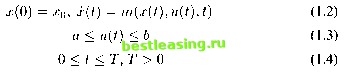

control problem which can be found in references [1, 1988], [5, 1975], and [8, 1983]. However, for a large class of reasonable cases, there are often no available results from standard theories. A more acceptable method is needed. In Blatt [2, 1976], there is some cost added when switching the control. The cost can be wear and tear on the switching mechanism, or it can be as the cost of loss of confidence in a stop-go national economy . The cost is associated with each switching of control. The optimal control problem in financial decision making with a cost of switching control can be described as follows:

subject to:

MINJ = J(u) + k-y = Г f(x{t),v{t),t)dt + k-y (1.5)

x(0) = x0,x(t) = m(x(t),u(t),t) (1.6)

u(t) = piece-wise constant with at most N jumps (1.7)

0<t<T, T>0 (1.8)

к < N, the control jumps (1.9)

Here, is the positive cost. is an integer, representing the number of times the control jumps during the planning period [0, T]. In particular, и may be a piece-wise constant, thus it can be approximated by a step-function. Only fixed-time optimal control problems are considered in this book which means T is a constant. Although time-optimal control problems are also very interesting, they have not been considered in this research.

The essential elements of an optimal control model (see Islam [36, 2001]) are: (i) an optimization criteria; (ii) the form of inter-temporal time preference or discounting; (iii) the structure of dynamic systems-under modeling; and(iv) the initial and terminal conditions. Although the literature on the methodologies and practices in the specification of the elements of an optimal control model is well developed in various areas in economics (such as optimal growth, see Islam [36, 2001]; Chakravarty [9, 1969]), the literature in finance in this area is not fully developed (see dynamic optimization modeling in Ta-perio [81, 1998]; Sengupta and Fanchon [80, 1997]; Zieamba and Vickson [89, 1975]). The rationale for and requirements of the specification of the above four elements of dynamic optimization financial models are not provided in the existing literature except in Islam and Craven [38, 2002]. In the present study, the main stream practices are adopted: (i) an optimization criteria (of different types in different models); (ii) the form of inter-temporal time preference-positive or zero discounting; (iii) the structure of dynamic systems