

|
|

|
Промышленный лизинг
Методички
umO = (um0i,um02, ,umQnn), and vector ul = lower bound of um, vector uu = upper bound of um, thus uu < um < ul. Initialize the value of the state function xinit. Step 2. Call the MATLAB constr function. In turn, constr calls the Minimizing Program to calculate the minimization of the calling program with respect to the optimal vector um. Step 3. Input the optimal result um into Minimizing Program again to obtain the results of the objective function Jnn (the last value of the calculation) and the state vector xm, corresponding to the optimal um. Step 4. Attach a cost К to nn. Add К *nn to the objective function (2.7) and calculate Step 5. Set a bigger nn; then go back to Step 2; EXIT when the result of cost function J stops decreasing. Algorithm 2.2: Minimizing Program (see project1 2.m in Appendix A.1) Step 1. Initialization. Input vectors um, par and initial state xinit. Set the initial state xm(1) = xinit, and nx = par(1), the number of the state components, nu = par(2), the number of the control components; initialize scaled time t = 0, subinterval counter it =1, hs= 1/nn(length of each equal subinterval). Choose the Input function for dynamic equation as the right side of equation (2.9) to calculate the differential equation, input um. Step 2. Call SCOM package function nqq with the stated Input function for dynamic equation to solve the differential equation (2.9) of the state function x(t). Tabulate the solutions as the components of the vector xm = Step 3. Set the initial state zz = 0. Set initial scaled time t = 0, subinterval Step 4. Call SCOM function nqq with the stated Input function for integration calculation to calculate: where: h = l/nn when: jh<r < (j + l)h by solving the differential equation: w(0) = 0,w(t) = M(r)) - <j>(<p(T))]2h-l(tj+1 - tj)} when: jh<r < (j + l)h Tabulate the results in w(.) as the components of vector jm = [j(l),...,j(nn)}. Step 5. Take the last result of the vector jm as the value of the objective function, and calculate the constraint function of Minimizing program , which is: g(um) = urrii - 1. Algorithm 2.3: Input function for dynamic equation (see project1 3.m in Appendix A.1) Step 1. Initialization. Input scaled time t, subinterval counter it, the length of subintervals hs, and vector um, and set the number of subintervals nn = 1 /hs. Step 2. Set the control policy as vector и = [u(l),u(2),..., u(nn)\ with alternating values 1 and 0 (as in 2.10) in successive subintervals. Step 3. Construct the right side of the differential equation for the state function using the piecewise-linear transformation in (2.5). Algorithm 2.4: Input function for integration calculation (see project1 4.m in Appendix A.1) Step 1. Initialization. Input scaled time t, subinterval counter it, the length of subintervals hs, vector xm representing the values of the state function at each switching time, and also a new initial state zfor integral, and the vector um. Set the number of subintervals nn = 1/hs. Step 2. Use the linear interpolation to get an estimate xmt of the state, in a time between grid-points where Step 3. Add up components of the lengths of the switching time intervals in um to obtain the switching times in (2.4). Step 4. Construct the right side of the equation (2.4) to obtain the time variable t. Step 5. Calculate the integral in (2.6) at scaled time t. When the number of switching time N increases, the cost function decreases because of the better approximation. While calculating a minimization problem KN + , v, the term KN increases with N increasing, and Jjv decreases with bigger N. It can be found that the cost of changing control is very critical in the cost function. A proper chosen cost K will efficiently lead the cost function to the minimum. The analysis of the cost will be discussed in later sections. 7. An Investment Planning Model and Results In this section, the computational results reported by a set of graphs will be introduced to verify the algorithms developed in Section 2.6. First we will introduce the fitting function. In this example, the fitting function is set to be The state function is used to approximate this fitting function. The formulae for this financial optimal control model is shown as follows: subject to: 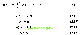 where x(t) = stock price, u(t) = the proportion of total investment in stocks compared to other forms of financial investment. Although the above model is an illustrative model, it can, however, represent an interesting financial decision making problem. The state equation represents the dynamics of the price of a stock. It is assumed that the change in the price of a stock is determined by the proportion of allocation of total funds for purchasing a stock. The objective of this control problem is to determine the value of u(t) (which only takes the value of 1 or 0) which can optimize the objective function so as to minimize the deviation of the state variable from its target value specified. Therefore this model (2.11 to 2.15) is an investment planning model with some sub-utilization criterion included in the model. The target function is 0.4*£2. First set n = 2 (n is the number of time intervals), and control takes as 1,0 in time intervals The model 2.11 to 2.15 was solved with these parameter values and the results are shown 1 2 3 4 5 6 7 8 9 [ 10 ] 11 12 13 14 15 16 17 18 19 20 21 22 23 24 25 26 27 28 29 30 31 32 33 34 35 36 37 38 39 40 41 42 43 44 45 46 47 48 49 50 51 52 53 54 55 56 57 58 59 60 61 62 63 64 65 66 67 |