

|
|

|
Промышленный лизинг
Методички
in Appendix B.l and are represented by Figure 2.1. In Figure 2.1, it is shown that during the planning horizon [0,1], the control only jumps once at time t = 0.127. The state vector xm takes the value [0.127, 0.127] at the grid-points of two subintervals [0, 0.127] and [0.127, 1]. The approximation between the state function xm and the fitting function 0.4 * t2 is not very good when the number of the switching times is quite small (n is only 2). *- represents the state function x(t) and . represents the fitting function 0.4 * t2 in the following graph.  о oi a.l a.a c.4 os at ar t.a at i гпит Figure 2.1. Plot of n=2, forcing function ut=1, 0 Then increase n to 4. During the whole time [0,1], the control jumps three times. A better approximation is shown in Figure 2.2 with more jumps of the control. 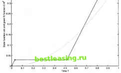 Figure 2.2. Plot of n=4, forcing function ut=1,0,1,0 Set n = 6, and run the program. A much better approximation than n = 4 is shown in Figure 2.3 because of the increased switching times. рки Qt пы§. Югопд <ul* 1,0,1,0,1,0 Mi-1-1-1-1-1-1-1-1-1-!  О 0.1 ftZ 0.3 0.4 0.5 0.6 D7 O.S 0.0 f Figure 2.3. Plot of n=6, forcing function ut= 1,0,1.0,1,0 When n - 8, a very close fit between state xm and the given fitting function ф(г) is shown in Figure 2.4. The result proves a very good convergence of the algorithms. 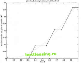 Figure 2.4. Plot of n=8, forcing function ut= 1,0,1,0,1,0,1,0 In Figure 2.5, although the approximation between xm and ф(Ь) is still getting better when the difference between the result of and is not as big as between and The decreasing of the results of the objective function slows down when is very large. pit* of rixl 0. tijfC* lUfiCllon ш= 1.0.1.0.1.0.1,0,1 -0 0.41--i-г- -i-1-1-1-1- 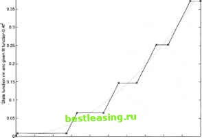 0 0.1 0.2 0.3 0.4 0.Б 0.6 0 7 0$ 0.9 1 Тьп T Figure 2.5. Plot of n=10, forcing function ut= 1,0,1,0,1,0,1,0,1,0 The results of the objective function according to different numbers of the time intervals n are put in Table 2.1. The decreasing of the results of the objective function follows the increases number of the time intervals When is small, the result of the objective function will decrease very fast, however this decrease will slow down when becomes big. A good illustration is shown in Figure 2.6. Table 2.1. Objective functions with the number of the switching times 2 0.062696 4 0.029085 6 0.018364 8 0.013369 10 0.010463 In Figure 2.6, the results of the objective function against the different number of the time intervals are shown. From the graph, we will find out that the descent of the results of the objective function slows down when the number of time intervals n increases. The conclusion can be made that more jumps of the control in the time period [0, 1] give abetter association between the state x(t) and fitting function (i.e. makes the financial system more stable along 1 2 3 4 5 6 7 8 9 10 [ 11 ] 12 13 14 15 16 17 18 19 20 21 22 23 24 25 26 27 28 29 30 31 32 33 34 35 36 37 38 39 40 41 42 43 44 45 46 47 48 49 50 51 52 53 54 55 56 57 58 59 60 61 62 63 64 65 66 67 |