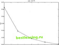Figure 2.6. Plot of the values of the objective function to the number of the switching times

The optimal control problem in (2.11)-(2.15) is computed and the results are shown in the above graphs. The number of time intervals n - 2,4,6,8,10 is set consequently. A better fit comes into being Figures 2.1, 2.2, 2.3, 2.4 and 2.5. In Figure 2.6, it is shown that the result of the objective function J decreases while the number of time intervals increases. Same results are also shown in Table 2.1. Now a proper cost K is set and attached with the number of the time intervals nto the objective function J. The objective function (2.11) becomes:

MIN F = J(n) + kn = fl \x(t) - 0.4 *t2\dt + Kn (2.16)

Use the algorithms to solve this new optimal control problem with the same constraints as in (2.12)-(2.15). Three different values of cost К are chosen for F(n) = J(n) + К *n. The results of adding К * nto the objective function are shown in Table 2.2, corresponding to n = 2,4,6,8,12.

Table 2.2. Costs of the switching control attached to the objective function

its desired path) and leads the financial system to reach the best fit when n becomes infinity.

From the results in Table 2.2, a conclusion can be made that only when cost K takes a certain value, it will lead the cost function to a minimum infinite switching times. When К = 0.02, the results of the cost function are increasing from to and the increases become faster. When

K = 0.0002, the results are decreasing, but this decrease begins to slow down when increases. It is conjectured that when the number of the switching times is getting very big, this decreases will stop at a certain value of Meaningful results from К = 0.002 are given, and a minimum is obtained at n = 8. The following Figure 2.7 shows the results of the cost function against the number of the time intervals n while the cost K = 0.002 is attached to the objective function. The bottom of the line in the figure is the minimum point

plol of the cost function to Ihe cos! of the swilctiing conlrol 0.071-1-1-1-,-,-1-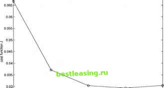

0.025

O.o;l---1----1-1-1

гэа56789 10

swik.tuxj time intervals

Figure 2.7. Plot of the cost function to the cost of switching control

This is an effective example of computational algorithms. All the results confirm the accuracy of computational algorithms in Section 2.6. A hand calculation of the part of the differential equation to exam the algorithms also gives a proof of computational accuracy. Some other experiments with different fitting functions will be discussed later in Chapter 5.

8. Financial Implications and Conclusion

The crucial aspect of the computational experiments undertaken here is that switching times and and the cost of switching times have significant implications for optimal investment planning. As the graphical results showed in Section 2.7, different numbers of switching times lead to different results for the objective function of the financial model. While the number of switching times increases, the value of the objective function decreases. That means a better fit is obtained. When a cost of changing control at each switching time is added to the original objective, the perspective changes. In the present case, when the number of switching times increases, the value of the term, which includes cost and the number of the switching, also increases. This increase slows down the decreasing of the original objective function. When the number of switching times increase to a certain value, the cost function stops decreasing and instead increases. The intermediate point between the decreasing and increasing is the optimal point.

The value of the cost of switching significantly influence the values of the switching times and optimal control. Comparing with the result of the objective function, if the cost is too big, the cost functional will increase all the time. It can be explained that it costs too much to change a control at each time interval. The financial system can never reach an optimal solution. But if the cost is too small, it could not affect the cost function at all. Then the control will jump infinitely in the time period to search an optimal solution, which is difficult to realize in real computation. Therefore, the value of the cost of switching time affects the optimal number of switching time. In terms of the value of the optimal control, it is found that several jumps in the strategy of investment in the stock market, shown by 1,0 values of investment in the stock market are optimal. A higher cost for switching reduces the optimal value of switching times compared to a situation when there is no cost for control switching.

An optimal investment strategy, therefore, should always be made on the consideration of the cost of control switching to determine how often the investment strategy can be changed between 1 and 0.

In the next chapter, a financial oscillator model for optimal aggregative investment planning will be presented. Since the oscillator problem has a state function, which is a second-order differential equation, the computational algorithms require transforming the second-order differential equation into two equivalent first-order differential equations. A new time scaled transformation for better integral calculation will be introduced in Section 3.3. The corresponding transformations of the state functions and the objective function will also be contained in Section 3.3. The computational algorithms for the financial oscillator problem will be described in Section 3.4. The computer software packages for these algorithms will be introduced in Appendix A.2. Different patterns of the control might lead the computation to different minimum