to solve the integration of the objective function (3.2). Input the vectors xm(: 1) and sm.

Step 5. Call SCOM function nqq with the stated Input function for the oscillator problem to solve the differential equation d(J(w(t)))/dt = - Tabulate results in as the components of vector

Step 6. Take the last result of the vector jm as the value of the objective function, and calculate the constraint function of Minimization program which is

Algorithm 3.3: Input function for second order differential equation (see project2 3.m in Appendix A.2)

Step 1. Initialization. Input scaled time t, subinterval counter it, the length of total subintervals hs and vector um. Set the value to parameters T, (set B for(3.18) and (3.19) in the next section). Set the number of the total subintervals nn = 1 /hs.

Step 2. Obtain the number of the big time intervals by nb = nn/ns for establishing the control policy.

Step 3. Set the control policy as vector и = [u(l),u(2),..., u(nb)] with alternating value 1 and -1, see (3.8); the control only jumps at the end points of the big time intervals.

Step 4. Construct the right side of the transformation equation for time pt in (3.10): pt = ф (r ) = nb~ 1 * (ptj+i - ptj) * (r - nb * (j - 1 )) + ptj , for ih < r < (г + l)h, ptj < t < ptj+\.

Step 5. Obtain the right sides of the differential equations by using the transformations in (3.13) and (3.14): x\(t) = х\\ф(т))(й/йт)ф{т) = T* x2{t)*nb*(ptj+\ -ptj), x2(t) = х2(ф(т))(ё/ёт)ф(т) = T*(-xi(t) + Uj - Г * х2(т)) * nb * {ptj+i - ptj) .

Algorithm 3.4: Input function for the oscillator problem (see project2 4.m in Appendix A.2)

Step 1. Initialization. Input scaled time subinterval counter it, the length of total subintervals hs, vector xm of values of first state function at switching times, and also the initial state z and vector sm. Set the number of the total subintervals nn = 1 /hs.

Step 2. Use linear interpolation to get the estimate xmt of the state, in a time between grid points where

Step 3. Add up the time intervals sm to get time tj in (3.9): t - <p(r) - h~1*(ti+i-ti)*{t-h*(i-\))+ti, forih < т < {i + l)h, ii < t < ij+i-

Step 4. Construct the right side of the equation (3.9) to obtain time variable

Step 5. Calculate the integrand in (3.15) at scaled time t: J = yj

5. Financial Control Pattern

The financial dynamic system introduced in Section 3.2 is a second-order differential equation, and the forcing function /indexforcingfunction u(t) takes values such as -2, 2, -2,2,..., switching between them at optimal switching times determined by an optimization calculation. Note if is restricted to choose two values -2 and 2, then both the patterns -2,2, -2,2,... and 2, -2,2, -2,... have to be computed. The comparison of the solutions of these two patterns will be discussed in next section. This research studies a set of bang-bang controls that jump on the extreme points of the feasible area. However, since the sequences of the control switching are not defined, all the sequences of the control patterns need to be computed and analyzed. A numerical example in financial modeling is shown next.

6. Computing the Financial Model: Results and Analysis

In this section, the control u(t) is set to be -2 and 2. The solutions of two different initial starts of control are discussed and compared. We can formulate the financial optimal control problem as follows:

subject to:

Xl(t)+T:

u(t) takes value - 2,2,... or 2, -2,... in successive time intervals (3.19)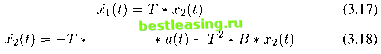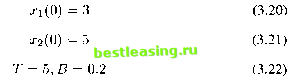

The target value of the target = Ы - 5.

Computational results are indicated in Table 3.1 above.

All the graphs shown below and on the following few pages are the computing results of the financial optimal control problem (3.16)-(3.22). There are three sets of the graphs, which represent the solutions at nb = 2, nb = 4, and nb = 6, where nb is the number of the big time intervals. In each set, the big time interval is subdivided by ns = 1,2,4,6,8,10 respectively, where ns is the number of the small time intervals. Each set has six pairs of graphs representing six different subdivisions. All the graphs are shown in the same order. A pair of graphs represent the statefunction x\(t) and the given fitting function againsttime t and the comparison of two state functions, x\(t) and x2(t).

plol of nb=2,nS 1. forcing function ul=-2 2 5j-г-1-1-1-1-г-1-г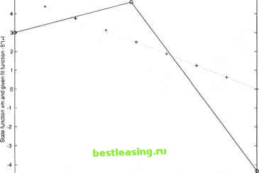

я I i i i i i i i i i I

0 0.1 0.2 03 04 0.5 0.6 0 7 0-6 09 1

Time T

Table 3.1. Results of the objective function at control pattern -2,2,...