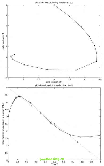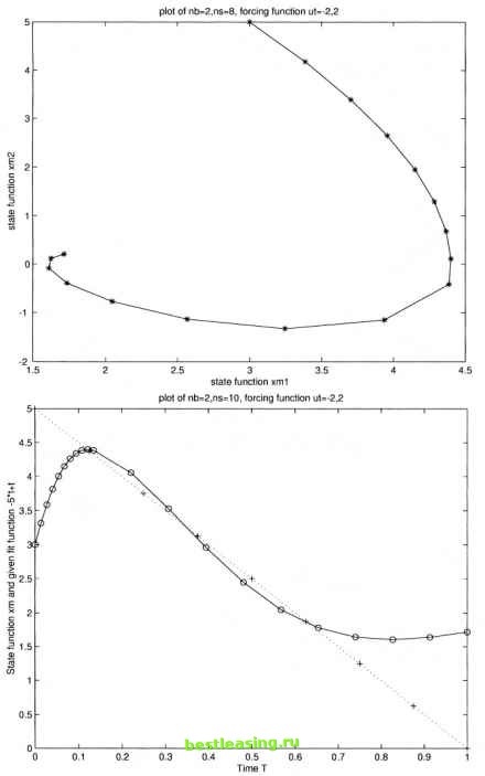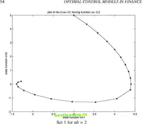The first set of the graphs is the solution at nb (the number of big time subintervals) equals 2. The time period [0,1] is divided into [0,t\] and [t\, 1]. ns (the number of small time subintervals) takes 1,2,4,6,8,10 respectively. As mentioned in Section 3.3, the control policy allows the control only to jump at the end points of the big time intervals (so the control does not jump at the end of the small time intervals). The control takes value -2,2 in two big time intervals and switches once at time The first pair of graphs

are the results of nb = 2 and ns = 1, that is, the time period is divided by 2 big intervals and each subinterval has no further subdivision. It is obvious that the approximation between state and the given fitting function is not very close because of the small nb and ns. As ns (the number of small intervals) increases, a better approximation is obtained. But since control only jumps once during the whole time horizon, it is hard to reach the global minimum. It is understandable that more jumps are helpful for searching a better fit - to find a more stable financial system. Although the ns still increases, the decreasing of the objective function slows down, thus nb needs to be increased. The results are also reported in Table 3.1. These results demonstrate the complexities of the dynamics of the financial system with damped oscillator.