

|
|

|
Промышленный лизинг
Методички
under modeling (different types - linear and non-linear); and (iv) the initial and terminal conditions - various types in different models. Optimal control models in finance can take different forms including the following: bang-bang control, deterministic and stochastic models, finite and infinite horizon models, aggregative and disaggregative, closed and open loop models, overtaking or multi-criteria models, time optimal models, overlapping generation models, etc.(see Islam [36, 2001]). Islam and Craven [38, 2002] have proposed some extensions to the methodology of dynamic optimization in finance. The proposed extensions in the computation and modeling of optimal control in finance have shown the need and potential for further areas of study in financial modeling. Potentials are in both mathematical structure and computational aspects of dynamic optimization. These extensions will make dynamic financial optimization models relatively more organized and coordinated. These extensions have potential applications for academic and practical exercises. This book reports initial efforts in providing some useful extensions; further work is necessary to complete the research agenda. Optimal control models have applications to a wide range of different areas in finance: optimal portfolio choice, optimal corporate finance, financial engineering, stochastic finance, valuation, optimal consumption and investment, financial planning, risk management, cash management, etc. (Tapiero [81, 1998]; Sengupta and Fanchon [80, 1997]; Ziemba and Vickson [89, 1975]). As it is difficult to cover all these applications in one volume, two important areas in financial applications of optimal control models - optimal investment planning for the economy and optimal corporate financing - are considered in this book. 2. (Karush) Kuhn-Tucker Condition The Kuhn-Tucker Condition condition is the necessary condition for a local minimum of a minimization problem (see [14, 1995]). The Hamiltonian of the Pontryagin maximum principle is based on a similar idea that deals with optimal control problems. Consider a general mathematical programming problem: MIN/(aO subject to: 9i(x) <0 92(x) < 0 (1.10) (1.11)  The Lagrangian is: L(x) - f(x) + \igi(x) + \2g2(x) + ... + \mgm(x) +Hihi(x) + /U22() + + /J-rhr(x) The (Karush-) Kuhn-Tucker conditions necessary for a (local) minimum of the problem at x = x* are that Lagrange multipliers Aj and /Xj exist, for which x* satisfies the constraints of the problem, and: VL(.x*) = 0; (1.17) Ai > 0,A2 > 0,...,Am > 0; (1.18) Ai5i(a;*) = 0,nihi(x) = 0,. ..,Xmgm(x*) = Q,vmhm = 0,...; (1.19) The inequality constraints are written here as then the corresponding at the minimum; the multipliers of the equality constraints can take any sign. So for some minimization problems where the inequality constraints are represented as the sign of the inequalities should be changed first. Then the KKT condition can be applied. The conditions for global minimum are that the objective and constraint functions are differentiable, and satisfy the constraint qualifications and are convex and concave respectively. If these functions are strictly convex then the minimum is also a unique minimum. Further extensions to these conditions have been made in the cases when the objective and constraint functions are quasi-convex and invex (see Islam and Craven [37, 2001]). Duality properties of the programming models in finance not only provide useful information for computing purposes, but also for determining efficiency or show prices of financial instruments. 3. Pontryagin Theorem The Pontryagin theorem was first introduced in Pontryagin [69, 1962]. Consider a minimization problem in finance given as follows: T is planning horizon, subject to a differential equation and some constraint: Here (1.23) represents the differential equation. (1.24) represents the constraint on control Let the optimal control problem (1.22) reach a (local) minimum at (х,й) with respect to the Li-norm for u. Assume that / and m are partially Frechet differentiable with respect to uniformly in near The Hamiltonian is shown as follows: with boundary condition. (b) the associated problems minimize at for all except at a null set. 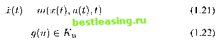 The necessary conditions for the minimum are: (a) a co-state function satisfies the adjoint differential equation: 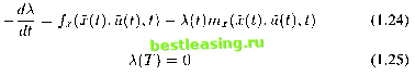
1 [ 2 ] 3 4 5 6 7 8 9 10 11 12 13 14 15 16 17 18 19 20 21 22 23 24 25 26 27 28 29 30 31 32 33 34 35 36 37 38 39 40 41 42 43 44 45 46 47 48 49 50 51 52 53 54 55 56 57 58 59 60 61 62 63 64 65 66 67 |