

|
|

|
Промышленный лизинг
Методички
This set of the graphs is the graphical solution at nb = 4 and ns = 1,2,4,6, 8,10. The control policy is u(t) = -2,2, -2, 2 in successive time intervals [0,t\], [ii,2], [*2>*з], [*з> 1] and control jumps three times at ti,t2, *з- A better approximation than the results at nb = 2 is shown. Most of the results confirm the computational algorithms 3.1-3.4 except a typical case nb = 4, ns = 8. In this case, the value of the objective function is bigger than the value of the objective function at nb = 4, ns = 6. That means the decrease of the objective function stopped at this point and increased instead. We also discovered that the value of the objective function at this point is same as the value of the other control pattern 2, -2, 2, -2 at the same point. They are shown in Table 3.1 and Table 3.2. From this test, it may be conjectured that the optimal search stops at a certain point for some reason. A small test was also made in the experiment, another control policy, which was created as u(t) = -2.05, 2, -2.05,2, was put into the program to replace the old control policy. A better search was obtained and the value of the objective function of the financial model became J = 0.2034. The new control policy enables the optimal search to continue until the optimum is reached. 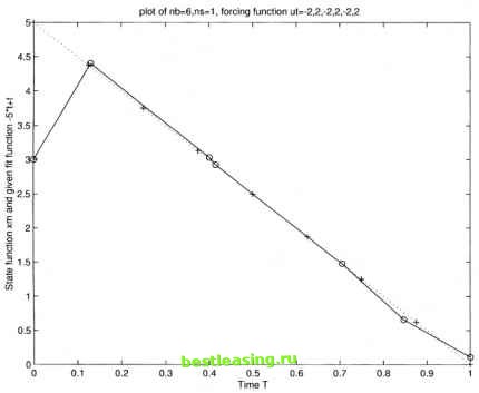 ptot of nb=6,ns=1, forcing function ut -2,2,-2,2,-2,2  2 I-1-1-1---1--1-1-1 0 0.5 1 1.5 2 2.5 3 3.5 4 4.5 state function xmi plot of nb=6,ns=2, forcing function uh.-2,2,-2,2,-2,2 5+--1-1-1-1-1-1-1-1-1-1 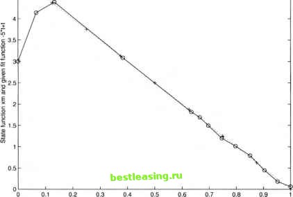 Time T 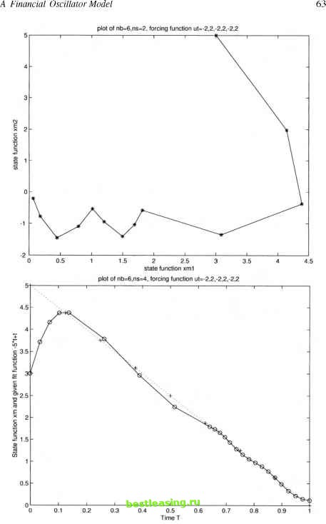
1 2 3 4 5 6 7 8 9 10 11 12 13 14 15 16 17 18 19 20 [ 21 ] 22 23 24 25 26 27 28 29 30 31 32 33 34 35 36 37 38 39 40 41 42 43 44 45 46 47 48 49 50 51 52 53 54 55 56 57 58 59 60 61 62 63 64 65 66 67 |