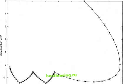2 1-1-------i--1-1-1-1 i i I

0 0 5 1 1.5 2 2.5 3 3.5 4 4 5

stale function xmt

Set 3 for nb = 6

This is the set of the graphical results at nb = 6 and ns = 1, 2, 4, 6, 8, 10. A better approximation than nb = 4 is obtained as expected. A similar computation as in case nb = 4, ns = 8 happened at case nb = 6, ns = 8 and case nb = 6,ns = 64. In case nb = 6,ns = 8, the optimal switching times are ii = 0.129, t2 = 0.709, t3 = 0.999, U = h = t6 = 0.999, fhe control stays at -2 from the third subinterval until the end of the time period. Although the control policy was set to switch five times in the program, the real computation did not show that the control jumped so often. As in the experiment we did for case nb = 4, ns = 8, this problem also can be solved by perturbing the control by a small amount. From the results shown in the Table 3.1, a conclusion can be made that when the number of big intervals and small intervals increases, the result of the objective function decreases. Although there are some unexpected results, a small disturbance of the control can easily obtain the correct answers. The experiment gave some promising results which confirm the accuracy of the computational algorithms in this chapter.

Another experiment is also presented to indicate the effects of the different patterns of the control.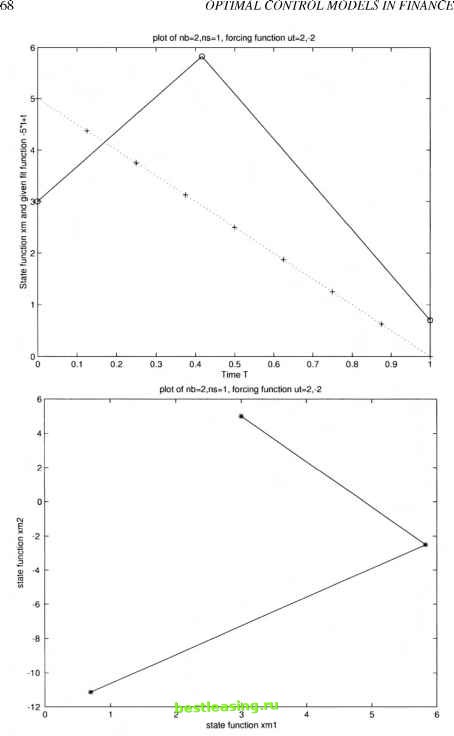

plol of nb=2,ns=2, forcing I unction ut=2,-2 6 ~-1-1-1-1-1-1-1-1-г

.2 I-1-1 I I I I L I J J

0 01 02 0.3 0.4 0.5 0.6 0.7 0.B 0.9 1

TimeT

plot of (10=2,ns=2, forcing [unction ut=2,-2 S j-г-- -1-1-1-+-1-1---n