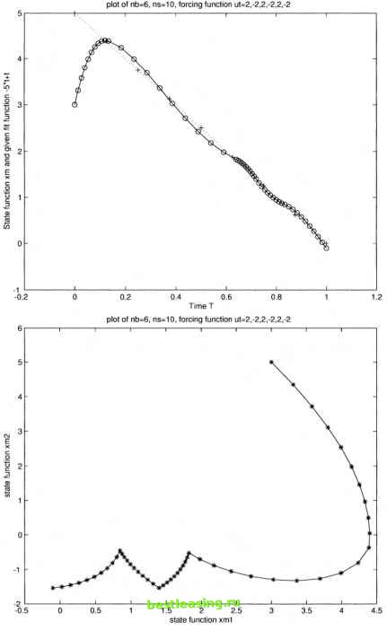Set 3 for nb = 6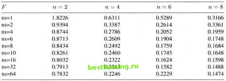

In this group of graphs, the pattern of control is 2, -2,2, -2,.... Like the previous experiment, this experiment starts from nb = 2, ns = 1 and increases nb and ns gradually. As expected, better approximation is obtained by increasing either nb or ns. Unexpected answers were also found at certain points. A small perturbation is helpful to gain the accurate results. Here, we only put the attention on the comparison of these two different patterns of the control. From Table 3.1 and Table 3.2, it is found that the values of the objective function of two different control patterns at starting points (nb = 2, ns = 1) have big differences. Pattern -2,2,-2,2,... gives much better result than pattern 2, -2, 2, - 2, It is an interesting phenomenon that when nb and ns become very big (more jumps and better gradient), the results of the objective function with different control patterns are very close. We can conclude that when optimal control jumps infinitely and the integration calculation has more subdivisions of the time period, the better fit for the problem can be reached whatever pattern of the optimal control is used.

Figure 3.1 and Figure 3.2 show the results of the objective function against 1/ns at two different control patterns. The value of the objective function tends to zero when the number nb of subdivisions increases. It is also confirmed that a greater number of subdivisions of the time interval will lead to a better integral calculation. The three lines in each figure also show that more jumps of the control will give better approximation. In the next figure, a cost is added to the objective function. A complete description of the cost of switching control has been discussed in Chapter 2. In this chapter, a cost is only attached to the number of large subintervals concerned with the control jumping, shown as follows:

K is the cost of changing control, nb is the number of large subintervals. In this computation, K is set to be 0.01, and ns = 64 for the accuracy of the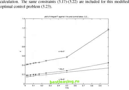

Figure 3.1. Plot of integral F against 1/ns at ut=-2,2

PloloF integral (against 1/ns and control takes 2.-2.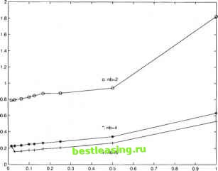

1/ns

Figure 3.2. Plot of integral F against 1/ns at ut=2,-2