4. Bang-Bang Control

In some optimal control problems, when the dynamic equation is linear in the control u(t), bang-bang control (the control only jumps on the extreme points in the feasible area of the constraints on the control) is likely to be optimal. Here a small example is used to explain this concept. Consider the following constraints on the control:

In this case the control is restricted to the area of a

triangle. The control, which is only staying on the vertices of the triangle and also jumping from one vertex to the other in successive switching time intervals, is the optimal solution. This kind of optimal control is called bang-bang control. The concept can also be used to explain a control:

where the optimal control
only takes two possible cases or depending on the initial value of the control. This control is also a bang-bang control.

In this research, only bang-bang optimal control models in finance are considered. Sometimes, a singular arc (see Section 1.5) might occur following a bang-bang control in a particular situation. So the possibility of a singular arc occurring should always be considered after a bang-bang control is obtained in the first stage.

5. Singular Arc

As mentioned earlier, when the objective function and dynamic equation are linear in the control, a singular arc might occur following the bang-bang control. In that case, the co-efficient of control in the associated problem equals zero, thus the control equals zero. So after discovering a bang-bang control solution, it is necessary to check whether a singular arc exists.

In what kind of situation will the singular arc occur? Only when the coefficient of in the associated problem may happen to be identically zero for some time interval of time say The optimum path for such an

interval is called a singular arc; on such an arc, the associated problem only gives A singular arc is very common in real-world trajectory

following problems.

0 < ui(t) + u2(t) < 1

m(t) > 0,u2(t) > о

a < u(t) < b

6. Indifference Principle

In Blatt [2, 1976], certain financial optimal control models that are concerned with optimal control with a cost of switching control were discussed, and an optimal policy was proved to exist. Also, the maximum principle of the Pontryagin theory was replaced by a weaker condition theorem ( indifference principle ), and several new theories were developed for solving the optimal control problems with cost of changing control. This research is dealing with an optimal control problem with a cost of changing control. Although the indifference principle theory is not being employed for solving the optimal control problems in this study, it is still very important to be introduced for understanding the ideas of this research.

Consider a financial optimal control model as follows:

where or 1 is the control setting at time the non-negative

integer к is the number of times control alters during time horizon T; and the are the times at which control alters, satisfying:

subject to: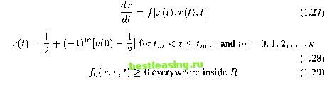

Let:

Given the policy P, the control function u(t) is shown in (1.30). Now the Hamiltonian of the Pontryagin theory is constructed as follows:

tf (A, x, v, t) = X(t)f(x, v, t) - / (ж, v, t)

(1.32)

The co-state equation is:

The end-point condition:

Theorem 2. An admissible optimal policy exists. See proof in reference [2, 1976].

Theorem 5. The indifference principle:

Let P(1.32) be an optimal policy. Let Я and X(t) be defined by (1.34), (1.35) and (1.36). Then at each switching time U of P(i = l,2,...,k). The Hamiltonian H is indifferent to the choice of the control, which is:

H(X(U),x(ti),l,ti) = H(X(ti),x(U),0,ti)

(1.35)

The relationship between the maximum principle and the indifference principle is that the indifference principle can be implied by the maximum principle . The maximum principle makes a stronger condition, that is, the control is forced to switch by the maximum principle when the phase space orbit crosses the indifference curve (1.37), while the control is allowed to change by the indifference principle at the same point. That means the control can stay the same in a region of phase space and also be optimal. It is not allowed to change the value of control v until reaching the indifference curve (1.37) again. It is workable even though the new theory requires more candidate optimal control paths. When a cost of a switching control exists, the