

|
|

|
Промышленный лизинг
Методички
<5 = discount on share price resulting from flotation cost с = a positive constant denoting the responsiveness of the price to changes in earnings and dividends T = planning horizon of the optimal financing program x(t) = dx(t)/dt The objective function of this model is to maximize the present value of the owners shares. Expressed by an integral plus an end-point term: MAXP(T)epT + Г e~pt[l - ur(t)]rE(t)dt (4.1) subject to: 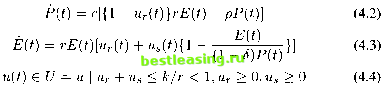 where, P(0) = Po, E(0) = E0 and the terminal condition is given by the fixed planning horizon T. Davis and Elzinga used the reverse-time construction technique which was given in reference [35, 1965], which will be described below, to systematically construct a complete solution from solution cases. The solution cases are classified according to the solution of a mathematical programming problem of each instant at time arising from the Maximum Principle [69, 1962]. 3. Analytical Solution Davis and Elzinga used the reverse-time construction technique that is particularly significant in solution synthesis. Starting from the terminal manifold and moving backwards in time, the entire space of state is filled with optimal trajectories solving the problem for arbitrary initial states. A linear program solved by inspection originally determined the solution of this model. The Maximum principle was successfully used and also modified to allow ease in handling discounted objective functional. The existence of the optimal control for this problem was established by corollary 2 of Theorem 4 in reference [50, 1967]: Theorem 4. Consider the non-linear process in Rn: (S) x = f(x, t, u) in Cl in Rn+l+m The data are as follows: 1. The initial and target sets Xo(i) and X\(t) are non-empty compact sets varying continuously in Rn for all t in the basic prescribed compact interval то < t < Ti. 2. The control restraint set t) is a non-empty compact set varying continuously n Rm for (ж, t) e Rn x [r0, n]. 3. The state constraints are (possibly vacuous) hl(x) > 0,..., hr(x) > 0, a finite or infinite family of constraints, where h1,..., hr are real continuous functions on Rn. 4. The family T of admissible controllers consists of all measurable functions u(t) on various time intervals to < t < t\ in [то, n] such that each u(t) has a response x(t) on to < t < steering ж(£0) € -Xo(io) to x(t\) e Xi(ii) andu( ) e Л1 ( (*)) 0,...,/1г(ж(£)) > 0. 5. The cost for each is: C(u) = g(x(h)) + / f(x(t), t, u{t))dt + t max *y(x{t)) Jt0 t0<t<ti where in and and are continuous in Assume: a. The family T of admissible controllers is not empty. b. There exists a uniform bound: \x(t)\ <bont0<t<ti for all responses to controllers c. The extend velocity set: V(x,t) = f°(x,t,u), f(x, t,u)\u € Q(x,t) is convex in Rn+1 for each fixed (x, t). Then there exists an optimal controller u*(t) on tg < t < t* in minimizing C{u). Corollary 2. Consider the control process in Rn: (S)x = A(x,t) + B(x,t)u with cost: C{u) = g(x{ti))+ / [A°(x(t),t)+B°(x(t),t)u(t)]dt+ess.sup j(x(t),u(t)) where: where the matrices A, B, A0, B° are C1 functions on Rn+1, g(x) and j(x, u) are continuous in Rn+m, and *y(x, u) is a convex function of и for each fixed x. Assume that the restraint set £l(x,t) is compact and convex for all (x,t). Then hypothesis c. is valid. If we assume 1. to 4. and a. b., then the existence of an optimal control on in is assured. Due to the Maximum Principle , the necessary conditions for to be optimal are: MAX ueUH where: грогЕе pt + сфр[гЕ +гЕфЕ{\ - jp]u pP] + гЕ[фЕ - сфр - фое pt}ur 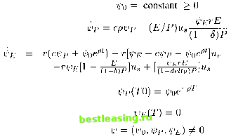 Here, o = l- The Hamiltonian can be modified by introducing new steady state variables Xp = ippept,\E = фЕерЬ- H = e~ptH = Я(А, P, E, u) = h(X, P, E) + 5r (A, P, E)ur + Ss (A, PE)ua (4.5) 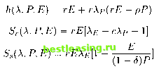
1 2 3 4 5 6 7 8 9 10 11 12 13 14 15 16 17 18 19 20 21 22 23 24 25 26 27 28 29 30 31 [ 32 ] 33 34 35 36 37 38 39 40 41 42 43 44 45 46 47 48 49 50 51 52 53 54 55 56 57 58 59 60 61 62 63 64 65 66 67 |