The adjoint variables are defined as follows: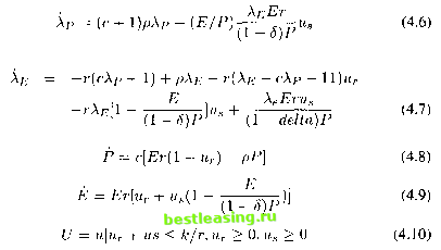

with boundary conditions P(0) = P0,E(0) = E0,\P(T) = 1,XE{T) = 0. Parameterizing terminal values of the state variables as P{T) = sp > 0 and E{T) = sE>0.

The maximization of H with respect to и can be characterized as follows: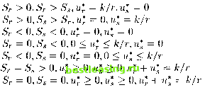

(a) (b) (c) (d) (e) (f) (g)

The synthesis of the solution was done by a construction technique in the reverse time sense. The complete solution is given as follows:

= 0,u*. = 0.

In the case (a)

A. u*

B. u* = k/r,u* = 0.

C. u* = 0, Ug = k/r

Л / r/n <- c+\c+(l-6)+l](k/p) 1-й rIP c(l-S)

The solution shows the classical bang-bang control. Although the singular arc cases appear in the synthesis, none of them are optimal. The computational methods established in Chapter 2 and Chapter 3 will be used to verify this solution in Section 4.6.

4. Penalty Terms

A substantial class of optimal control problems will deal with the terminal constraint as well as other constraints that may describe physical limitations on some process. For computational reasons, some penalty terms are required to be used to replace these constraints in order to obtain an unconstrained problem. There are some approaches with good reputations. Since the financial model discussed in this chapter has an end-point constraint on the market price of a share of stock at the end of the time planning horizon, the penalty term is used in the terminal constraint transformation. First an approach is introduced to deal with a minimization problem subject to both inequality and equality constraints:

MINj/(i) subject to g(x) < a, h(x) = b, where x e Rr [A]

Consider the objective function /(.) as a cost to be minimized; then additional penalty costs are added to /(.) when x does not satisfy the constraints. Define vector v+ = (vl + ,v2+,...,vn+) = v = (ы, v2, , vn) if vx, v2,..., vn > 0, 0 if v\,v2,... ,vn < 0. The problem (1) is replaced by the following unconstrained problem:

MINxf(x) + l-u \g{x) -a + /x 1 2 +l-u \\ \h{x) - b + ua] 2

The terms in g and h consist of the penalty functions. They are zero when x satisfy all the constraints, и is a positive parameter, that can more generally be replaced by different parameters for each component of and

and a are Lagrange multipliers. From the theory of augmented Lagrangian [14, 1995], this unconstrained problem with the penalty terms is minimized at the same point as the given constrained problem [A], provided that the Lagrange multipliers and are suitably chosen.

Before the penalty method of terminal constraints is stated, the Delta function should be introduced since it will be used to include the terminal constraints into the integral later. The Dirac delta function is described by:

<5(.) > 0, S(t) = 0 when t ф Oin R, and / 5{t)dt = 1.

Now consider an optimal control problem of the form:

МШх{Ш)Г°(х,и) := J f{x{t),u(t),t)dt + ${x(T))

A terminal constraint a(x(T)) = b can be replaced by a penalty term added to F°(x,u):

F(x,u) :=F°(x,u) + -u \\ Ф(х(Т)) - b* 2

where и is a positive parameter, and b* approximates to b, thus b* = b + в л, and where 9 is the Lagrange multiplier.

Thus an end-point term in a control problem can be included in the integrand as shown:

Г f(x(t), u(t), t)dt + Ф(х(Т)) = fF[f(x(t),u(t), t) + $>{x{t))5{t - T)]dt Jo Jo

and so is not an additional case to be treated separately.

A constraint such as J0l 0(u(t)) < 0, which involves controls at different times, can be treated by adjoining an additional state component:

Уо(0) = 0, yo{t) = e{u{t))

and imposing the state constraint yoiX) < 1- The latter can be handled by a penalty term where the parameter is small.

5. Transformations for the Computer Software Package for the Finance Model

In this section, in order to develop a computer software package of the optimal control for this financial model, some transformations of the formulas are introduced here to meet the requirement of the computation. Basically most transformation techniques with the division of time scales used here were introduced in Chapter 3. Only the different transformations for this particular computer package are introduced here.

The differential equations in (4.2) and (4.3) are represented as follows:

Р(т) = с[{1 - иг(т)}гЕ(т) - pP{tau)] *nb* (ptj+i - ptj) (4.11)