

|
|

|
Промышленный лизинг
Методички
Ё(т) = rE(t)[ur{t) + us(t){l- OPTIMAL CONTROL MODELS IN FINANCE E(t) {(l-S)P(t)} The integral in (4.1) is transformed as: ] *nb* (ptj+i-ptj) (4.12) 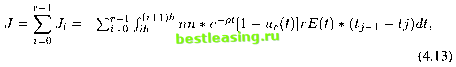 where Terminal state is treated separately for nqq package: Since in this model, time horizon parameter T is assumed to be greater than 1, another transformation of changing time interval [0, T ] to [0,1] is required for the program which only deals with the time period [0,1]. This transformation was indicated in section 2.3. Let a new time t equal here is the scaled time set for the computational methods. Then the differential equations and integral of objective function become: 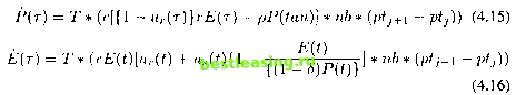 The integral in (4.1) is transformed as: 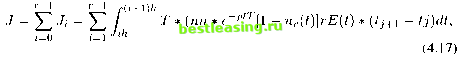 where h - 1/nn The transformations here only deal with the time variable t. The end-point term is considered separately in the program. 6. Computational Algorithms for the Non-linear Optimal Control Problem From section 4.3, we know that at a particular case (a), the bang-bang control is the optimal solution of the system. lies on the vertices of a triangular area: ur(t) > 0,?/.,(£) > 0; (4.18) ur(t) + ua(t) < k/r < 1. (4.19) However, a singular arc is possible, with u(t) lying on an edge of the triangle (instead of a vertex), when the parameters (p, c, r, etc.) of the functions take particular values. Since Davis and Elzinga did not have a computer software package for this optimal control problem, this research is focused on developing computer software based on the research work which has been done in Chapter 2 and Chapter 3. In order to get accurate estimates of the switching times, some computational methods have to divide [0, T] into many subintervals. The time transformation introduced by Goh and Teo [33, 1987] makes it possible to avoid this difficulty. The technique was also used to construct the computational algorithms in this section. We establish the control policy as bang-bang control here. The optimal switching times will be computed. Several sequences of the control patterns will be experimented with different initialization of the states. The results will be discussed and analyzed in next section. Computational method 4.1 Main Model Program (see model 1 1.m in Appendix A.3) Stepl. Initialization. First set the a vector of parameters = [p, k, r, d, c, t] which includes all the parameters in this financial model, p = is market capitalization rate, к = maximum investment rate, r = rate of return to equity, = discount on share price resulting from flotation costs, = a positive constant denoting the responsiveness of the price to changes in earnings and dividends, T = planning horizon of the capital budgeting program. Then set parameter par = [the number of the state components, number of control components, nb = the number of big subintervals, ns = the number of small subintervals, parameters]; and get the total number of the subintervals by calculating nn = nb* ns. Set the MATLAB constr function parameters par (13) = 1 (one equation, constraint in the minimization problem) , par(14) = the maximum number of function evaluations, and arbitrary starting lengths of the switching time intervals umO = (um0i,um02, итпь). Set the vectors of upper bounds uu and the vector of lower bounds ul of urn, thus uu < urn < ul. Also set the initial state xinit; Step2. Call the MATLAB constr function. In turn, constr calls the Model2 to calculate the minimization of the calling program with respect to the optimal vector um; Step3. Input the optimal result um to Model2 , to obtain the values of the objective function J(nn) (the last value of the integral) and state vector xm (xm is a vector of all the values of the state functions take at the grid-points of the switching time intervals). The result of the objective with respect to optimal switching times is the solution of this financial system model. Computational method 4.2: Model 2 (see model1 2.m in Appendix A.3) Stepl. Initialization. Input um, par and initial state xinit. Set the initial state xm(1, :) = xinit, and nx = par(1), the number of the state components, nu = par(2), the number of the control components (in this case, nx and nu both equal 2, there are two states and two controls,) nb = par(3), the number of big time intervals, ns = par (4), the number of small time intervals, nn = par(3) *par(4), the number of total time intervals, initial scaled time t = 0, subinterval counter it = 1, hs = length of the whole subinter-vals. Choose the Model3 as the right side of the differential equations (4.2) and (4.3), input um; Step2. Construct the vector sm whose components represent the lengths of the total time intervals by dividing each big time interval um by ns; Step3. Call the SCOM package function nqq with the stated Model3 to solve dynamic equations (4.2) and (4.3). Tabulate the solution for the state as the vector xm(: 1) = [xi(l),xi(2),...,xi(nn)],the result of (4.2), xm(: 2) = [2:2(1), £2(2), > 2(nn)], the result of (4.3); Step4. Set the initial scaled time t = 0, subinterval counter it = 1, initial state zz(: 1) = 0, ma = 1, the number of the input state function. Choose the Model3 for SCOM function nqq . Input the vector xm(: 1) and um; Step5. Call SCOM function nqq with the stated Model4 to solve the differential equation d(J{w(i)))/dt = - Tabulate the results in w(.) as the components of the vector 1 2 3 4 5 6 7 8 9 10 11 12 13 14 15 16 17 18 19 20 21 22 23 24 25 26 27 28 29 30 31 32 33 [ 34 ] 35 36 37 38 39 40 41 42 43 44 45 46 47 48 49 50 51 52 53 54 55 56 57 58 59 60 61 62 63 64 65 66 67 |