Step6. Obtain the last value xm(nn, 1) of the state vector for the end-point condition ;

Step7. Call the End-point condition to calculate the terminal state;

Step8. Add the result gained from End-point condition to the last value of the vector jm as the result of the objective function w(t) in (4.1), and calculate the constraint function of model2 which is g{um) = Ya=i umi - 1-

Computational method 4.3: Model 3 (see model1 3.m in Appendix A.3)

Stepl. Initialization. Input scaled time t, subinterval counter it, the length of total subintervals hs, vector um and vector par. Set the value of parameters p,k,r, d, c, T. Set the number of the total subintervals nn = 1/hs;

Step2. Obtain the number of the big time intervals by nb = nn/ns for constructing the optimal control policy;

Step3. Set the control policy as vector u= [щ, u2] which jumps between the vertices of the triangle area (4.18)-(4.19). The control only jumps at the end points of the big time intervals;

Step4. Construct the right side of the transformation equation for time pt in (3.10);

Step5. Obtain the right side of the differential equations by using the transformations in (4.15), (4.16).

Computational method 4.4: Model 4 (see model1 4.m in Appendix A.3)

Stepl. Initialization. Input scaled time subinterval counter it, the length of subintervals hs, vector xm of values of first state function at switching times, and also the initial state and vector sm. Set total subintervals nn = 1/hs;

Step2. Use linear interpolation to get the estimate xmt of the state, in a time t between grid points 0h, h, 2h,..., h * nn, where h = 1/nn;

Step3. Add up the time intervals sm to get time in (3.9);

Step4. Construct the right side of the equation (3.9) to obtain time variable Г;

Step5. Calculate the integrand in (4.17) at the scaled time t, and change the sign of the integral. (This problem is seeking for a maximum. Since the computer package only deals with minimization calculation, an opposite sign of the objective function needs to be changed.)

Computational method 4.5 End-point condition (see model1 5.m in Appendix A.3)

Stepl. Initialization. Input the last value of the first state function in vector xm and the parameters par which are required by the End-point condition ;

Step2. Construct the terminal term in (4.14).

7. Computing Results and Conclusion

In this section, the algorithms 4.1-4.5 are used in a computer software package (see in Appendix A.3) which was developed for this financial decisionmaking model (4.1)-(4.5). Before we present the computing results, the analytical solution in the Davis and Elzinga [22, 1970] finance model is described first for the future comparisons. Figure 6 in Davis and Elzinga [22, 1970] shows the optimum solution graphically, which means:

Solution case [1]: when -щ > cps, the optimal solution has control in case [C] all the time;

PCVS cr~\--с

Solution case [2]: when the optimal solution has control

switching from case [B] to [A] at a switching time.

The control regions [A], [B], [C] are described in Section 4.3.

First, set the parameters:

/&- = 0.1,fc = 0.15,r = 0.2,<J = 0.1,c = 1

which meets the restriction on in case (a) in Section 4.3.

1-5 0.9

c(l - 5)

Initialize the states:

P(0) = 3,E(0) = 2

Map the control (ur, us) in this order:

[B] [C] [A]

ur ur ur

к/г, us 0,us =

0, Uq =

= 0 k/r 0

in successive time intervals. [B], [C], [A] for nb = 3, or [B], [C], [A], [B], [C], [A] for nb = 6.

Then run the programs for the algorithms 4.1 -4.5 (details see modell l .m , modell 2.m , model1 3.m , model1 4.m , model1 5.m in Appendix A.3). All the cases are put into Table 4.1.

Table 4.1. Computing results for solution case [ 1 ]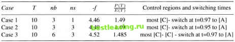

Here, most [C] indicates that most of the time is spent in [C].

From the results in Table 4.1:

Then according the analytical solution in Davis work, the optimal solution is supposed to be in solution case [1], which is control [C]. The computing results in Table 4.1 almost agree with the analytical solution. Since 1.49 is very close to 1.47, the case [A] will mix with case [C] at some point. This computed case is close to the theoretical optimum, but it does not exactly agree with it. Another solution case is verified next.

Initialize the states:

P(0) = 0.5, £(0) = 1