

|
|

|
Промышленный лизинг
Методички
Map the optimal control (ur, ua) in this order: [C] ur = 0, us - k/r [B] ur = k/r, us = 0 [A] ur = 0, us - 0 in successive time intervals. [C], [B], [A] for nb = 3, or [C], [B], [A], [C], [B], [A] for nb = 6. Then run the programs. The results are shown in Table 4.2. Table 4.2. Computing results for solution case [2]
From the result in Table 4.2: P(T) The computing results agree with the analytical solution in solution case [2], which is control case [B] switching to [A] at a certain switching time. In this example, the computed results agree well with the theory. Another example with the same initialization but a different given order of control mapping is given in Table 4.3; the results agree with Table 4.2. The optimal control are in order: [C] [A] Table 4.3. Computing results for solution case 2 with another mapping control 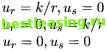 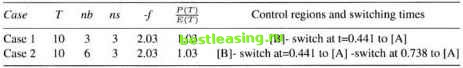 An approximate calculation using the SCOM package, dividing [0,1] into 20 equal subintervals, also confirms the switching patterns for solution case [2]. The following computation has the same initialization of the parameters as the above computation. The initial states also take: P(0) = 0.5, £(0) = 1. The solution of the computation is shown as follows. The optimal control takes values: (ur,us) = (k/r,0),(k/r,0),{k/r,0),(k/r,0),(k/r,0), (k/r,0),(k/r,0),(k/r,0),(k/r,0), (0,0), (0,0), (0,0), (0,0), (0,0), (0, 0), (0,0), (0,0), (0,0), (0,0), (0,0) The states are: P(T) = 1.99 E(T) = 1.96 The objective function is: -/ = 2.04 the optimal solution is expected to be in solution case [2] in the analytical solution. The results of this computation are very close to Table 4.2 and Table 4.3 and also confirm the analytical solution in Davis and Elzings finance model. The optimal control jumps from [B] to [C] at t = 0.45. The computation in this chapter agrees with the analytical solution in Davis and Elzinga [22, 1970]. The results might change if the parameters have been changed. The parameters set in this research are chosen to meet the restriction on г/pin case (a) (section 4.3). Further research on different parameters and more subdivisions of the time interval will be very interesting. 8. Optimal Financing Implications The results of this computation in Tables 4.2 and 4.3 are very close to the analytical results in Section 3 and also confirm the analytical solution in Davis and Elzinga [22, 1970]. The model results provide the dynamic structure of capital of a firm and the optimal switching time from moving from one source of finance to another. There is one switch in the firms financing strategy over the planning period. The levels of the two sources of fund depend on the relationships between the rate of return on equity capital and the investors discount rate and the relationship between the equity per share (E) and the market price of stock(P), thus the optimal control jumps from [B] to [C] at t = 0.45. Since the computational results of the optimal financing model are consistent with the analytical results derived in Section 3 and the results of Davis and Elzinga, they can be applied to understand optimal financing strategies of corporations to determine the optimal mix of structure of long-term funds to use in actual management of the capital structure of companies. Although theoretical controversies continue, model results suggest that the optimal structure which minimizes the firms composite cost of capital changes over time. The model results provide the timing of switching from one fund to another fund. In real life, these switches depend on the cost of these funds, the rate of return, share prices, debt capacity, business cycles, business risks, etc. Various results are generated by different sets of parameter values of the model. Sometimes subjective judgments need to be made to choose the appropriate optimal capital mix path of the firm. 9. Conclusion The determination of the optimal structure of corporate capital and the switching times for different methods of financing are essential for the actual management of capital structure of corporations. The computation of optimal switching time in this paper agrees with the analytical solution in Davis and Elzinga [22, 1970]. The results might change if the parameters are changed. The parameters set in this research is chosen to meet the restriction on r/p in case (a) (Section 4.3). Further research on different parameters and more subdivisions of the time interval will be very interesting. Development of an algorithm to coincide the time subdivisions with switching times are also another important area of further research. 1 2 3 4 5 6 7 8 9 10 11 12 13 14 15 16 17 18 19 20 21 22 23 24 25 26 27 28 29 30 31 32 33 34 35 [ 36 ] 37 38 39 40 41 42 43 44 45 46 47 48 49 50 51 52 53 54 55 56 57 58 59 60 61 62 63 64 65 66 67 |