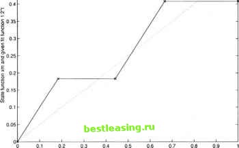
Chapter 5

FURTHER COMPUTATIONAL EXPERIMENTS AND RESULTS

1. Introduction

This chapter will give some experiments that have been done for examining the computational algorithms developed in Chapter 2 and Chapter 3 for computing dynamic optimization financial models. The computation tests for the algorithms in Chapter 2 are presented in Section 5.2. Three computing examples are included. The problems met during computation are discussed and the solutions for those problems are indicated. Section 5.3 contains a different control policy with one possible pattern of the financial optimal control problem (3.2)-(3.6). The computing results of this new control policy are also included. The objectives of the modeling experiments are to provide examples of additional modeling structures which can be adopted in financial modeling including some new forms of the objective functions and control patterns, and to test the computational algorithms and the computer program by applying them to some further models.

2. Different Fitting Functions

In this section, three different given fitting functions of OCPWCS (Optimal Control Problems When Control are Step functions) are indicated. The difficulty and non-accuracy in the computation of financial models are analyzed and the possible solutions of those problems are given.

2.1 Calculation with square criterion in the objective function

Consider a financial optimal control model as follows:

MINJ= [\x(t)-l/2t)2dt (5.1)

subject to:

x(t) = u(t) (5.2)

u(t) = 1 or 0 (5.3)

0 < t < 1 (5.4)

The target function is: 1/2*t.

Now apply the algorithms 2.1 - 2.4 to solve this problem. Note the objective function is no longer an absolute value. The algorithm 2.4 needs to be modified to meet the square value. The time division technique will be used here. The following graphs and tables are the computing results of this control problem. In the figures, *- represents the state function x(t), and . represents the given fitting function l/2i.

This model is the same investment planning model as in Section 2.7. However this model has a different fitting functions and the objective function is in a squared form which is a preferred form of decision criteria in economies (Islam [36, 2001]).

Figure 5.1 is the result of n = 4 (numbers of the time intervals).

plol ot л=4, forcing lundjon UU1,0,1 0.51-1-1-1-1-1-1-1-1-1-n

TlmeT

Figure 5.1. Plot of n=4, forcing function ut=1,0,1,0

The outputs of this computation are shown as follows: The real optimal switching times are:

vi = 0.183, v2 = 0.442, v3 = 0.667

Time period [0,1] is divided into four subintervals:

[0,0.183], [0.183,0.442], [0.442,0.667], [0.667,1]

The control is mapped as:

u(t) = 1,0,1,0 in successive time intervals

As results, the state variables of the financial system takes values as:

x(t) = 0.183,0.183,0.408,0.408 at the ends of the time intervals

The minimization of the objective function at is:

J = 0.0028

Figure 5.2 is the graph result of n = 10.