

|
|

|
Промышленный лизинг
Методички
plot of n 10, forcing function ut=1,0,1,0,1,0,1,0,1,0 0.51-1-1-1-1-1-1-1-г  0 0.1 0.2 0.3 OA 0.5 0.6 0.7 0.5 0.9 1 TimeT Figure 5.2. Plot of n=10, forcing function ut= 1,0,1,0,1,0,1,0,1,0 The outputs of n - 10 are: The real optimal switching times are: ui = 0.078, u2 = 0.190, u3 = 0.286, u4 = 0.381, u5 = 0.476, u6 = 0.572, v7 = 0.668, u8 = 0.763, u9 = 0.858 Time period [0,1] is divided into 10 subintervals: [0,0.078], [0.078,0.190], [0.190,0.286], [0.286,0.381], [0.381,0.467] [0.467, 0.572], [0.572, 0.668], [0.668,0.763], [0.763,0.858], [0.858,1] The control is mapped into: u(t) - 1, 0,1,0,1,0,1,0,1,0 in successive time intervals As results, the state takes values as: x(t) = 0.078,0.078, 0.174,0.174,0.270, 0.270, 0.366,0.366,0.460,0.460 at the ends of the time intervals J = 0.0005 When the jump of the control increases, abetter approximation between state x(t) and given fitting function is obtained. In this experiment, several other computations have also been done in the case of n = 2,6, and, 8. The results of the objective function of all these cases are shown in Figure 5.3 and in Table 5.1. The value of the objective function decreases when n increases. It is confirmed that the value of the objective function tends to zero when the control jumps infinitely often. 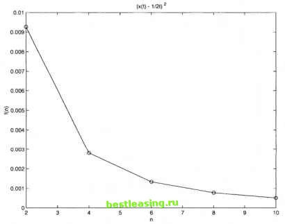 Figure 5.3. Results of objective function at n=2,4,6,8,10 The above results imply that for the development of a stable investment plan aimed at certain target value for the stock price, flexibility in switching among investment strategies is essential. The minimization of the objective function at n = 10 is: Table 5.1. Results of objective function at n=2,4,6,8,10 2 0.009259 4 0.002806 6 0.001335 8 0.000778 10 0.000508 2.2 Calculation with absolute value criterion in the objective function In this section, a similar financial model similar experiments as in Section 5.2.1 are introduced. The difference is that the objective function in this section is the absolute value of the state approximating the given fitting function. The financial optimal control problem is shown as follows: MINJ= С \x(t) - l/2t\dt Jo subject to: 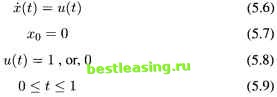 The definition of the variables and parameters are same as in Section 3.2. However the present model has a different forcing function. This is an optimal financing model for a firm where the decision problem involves whether to buy back (-1) or issue (1) some stocks or to maintain the present situation (0) of the amount of stocks used in the market so that the firms stock price remains stable. Apply the algorithms 2.1-2.4 on the problem (5.5)-(5.9). Only one modification is made in algorithm 2.4 for this given fitting function There are 1 2 3 4 5 6 7 8 9 10 11 12 13 14 15 16 17 18 19 20 21 22 23 24 25 26 27 28 29 30 31 32 33 34 35 36 37 [ 38 ] 39 40 41 42 43 44 45 46 47 48 49 50 51 52 53 54 55 56 57 58 59 60 61 62 63 64 65 66 67 |