two graphs shown as follows which represent n = 4 and n = 8 respectively. As in the last section, the lines represent state function by and given fitting function by

The results gained from n = 4 are shown as follows:

The real optimal switching times are:

ui = 0.142, v2 = 0.428, v3 = 0.714

Time period [0,1] is divided into four subintervals:

[0,0.142], [0.142,0.428], [0.428,0.714], [0.714,1]

The control is mapped into:

u(t) = 1,0,1,0 in successive time intervals

As results, the state variable of the financial system variable of the financial system takes values as:

x(t) = 0.142,0.142,0.4280.428 at the ends of the time intervals

The minimization of the objective function at n = 4 is:

J = 0.032

Figure 5.4 also shows the approximation between the state function x{t) and given fitting function l/2£. Three jumps of the optimal control are shown.

ptoloi Farcing lurcclion иы.0,1.0 0.Б,-1-1-1-1--1-1-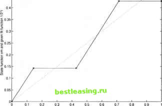

Figure 5.4. Plot of n=4, forcing function ut=1,0,1,0

An interesting situation was met during the computation at the case n = 8. Clearly the wrong result was gained in which the control only jumped once at and the minimum of the objective function was greater

than the value of the minimum at the case It is possible that the com-

putation was finding some local minimum, instead of the global minimum. A check for this mistake was also made. It was found that error was in the initialization of the lengths of time intervals umO. Originally umO was set as [1/2,1/2,1/2,1/2,1/2,1/2,1/2]. Since the constraint on timeHsO < t < 1, then the original set of um0 did not meet this restriction. It also misled the computation to a local minimum. The correct initialization of um is very critical for the whole computation. The mistake also occurred in the computation of the case n = 8 in Section 5.2.3. Now set um0 as Accurate results of the problem are shown as follows.

The real optimal switching times are:

i = 0.066, v2 = 0.199,из = 0.332, v4 = 0.465, v5 = 0.598, v6 = 0.731, v7 = 0.865

Time period [0,1] is divided into four subintervals:

[0,0.066], [0.066,0.199], [0.199,0.332], [0.332,0.465], [0.465,0.598], [0.598,0.731], [0.731,0.865], [0.865,1]

The control is mapped into:

u(t) = 1,0,1,0,1,0,1,0 in successive time intervals

The state takes values as:

x(t) = 0.066,0.066,0.199,0.199,0.332,0.332,

0.465,0.466,0.466 at the ends of the time intervals

The minimization of the objective function at n = 8 is:

J = 0.015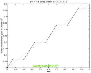

Figure 5.5. Plot of n=8, forcing function ut= 1,0,1,0,1,0,1,0

Figure 5.5 also shows a better approximation than n = 4.