The results of other cases at n - 2,6,10 are shown in Table 5.2. The value
of the objective function decreases when n (the number of the time intervals) increases.

Table 5.2. Results of objective functions at n=2,6,10

2.3 Problem of the fitting function with big slope

In this section, a special case is introduced where the fitting functions slope is greater than 1 at time t=l. Since the given fitting function is approximated by a piecewise-linear function with slope 1 and 0, the fitted function does not need any part of slope 0 near t = 0.6. In this case, the give fitting function has a slope 1.6 at t = 1, thus a slope 1 cannot give a good fit any more. A similar problem happened in Section 5.2.2 where the computation reached a local minimum also occurred at case

Consider the following optimal control model of finance: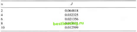

subject to: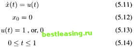

After running the program of the algorithms 2.1-2.4, two mistakes were found. First, the control stopped jumping at case n = 8. Second, the approximation did not work well at the slope close to 1.

The first problem was met while computing the optimal control problem (5.5)-(5.9). A different start of um can fix this problem. Here, we introduce several other methods to exam which one works well in the computation. First (method 1), simply divide each optimal um at case n = 4 by 2 as the initial start of um for case The idea behind this method is that if the com-

putation starts from a good minimum at the smaller jumps of control, it will also lead to a good minimum at the greater jumps of control. Second (method 2), since the non-accurate results always gave zero of um, which means no switching times, the lower bound of the um can be modified from the original zero to a very small number to avoid the situation of um = 0. Thus, the control jumps. It does not guarantee the computation will reach optimum. Sometimes these two methods can be combined together. Method 3, is the method used in Section 5.2.2 for solving a similar problem.

Using a control that can provide a bigger slope for the fitting function can solve the second problem mentioned earlier about the slope of the given fitting function. Method 4 lets control take a larger value to fit a function whose slope is great.

Figure 5.6 is the result of method 3. *- represents state function, . represents the fitting function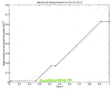

Figure 5.6. Plot of n=8, forcing function ut= 1,0,1,0,1,0,1,0

Table 5.3. Test results of the live methods

J is the value of the objective function. These five cases represent four methods described earlier. Case 1 is for method 1, Case 2 is for method 2, Case 3 is for the combination of method 2 and method 3, Case 4 is for method 3, and Case 5 is for method 4. Method 1 and method 3 both obtain similar results. This proves that the right initialization of um0 will help the computation searching the optimum. Method 2 did not give promising results in the test. It can be explained that certain time intervals are not optimal, so if the control is forced to jump in that period, the optimum will be skipped. Method 5 does solve the problem with a big slope of the fitting function.

2.4 Conclusion

The three experiments that have been done in Section 5.2.1, 5.2.2, 5.2.3 are very important for the computer package which was developed for solving a certain class of optimal control problems. They make the program more general, the results more accurate, and computation more stable. The optimal control problems when controls are step functions can be solved using this computer package. Only very small modifications are needed. The accuracy gained from these computational algorithms is also very useful for the algorithms 3.1-3.4 for oscillator problems.

3. The Financial Oscillator Model when the Control Takes Three Values

In this section, an experiment when the control takes three values is introduced to test the algorithms 3.1-3.4 in Chapter 3. The results of the problem are also analyzed.

The tests of all these methods are put in Table 5.3.