Table 5.4. Results of financial oscillator model

From the results in Table 5.4, a conclusion can be made that the subdivision of the time intervals is necessary especially when the nb (the number of the

3.1 The control takes three values in an oscillator problem

Consider the financial oscillator model as follows:

MINJ= t \xx(t) -4*sin(5t + l)\dt (5.15) Jo

subject to:

x\(t) = T*x2(t) (5.16)

x2(t) = -T*xl(t) + T*u(t)-T2*B*x2{t) (5.17)

u(t) takes value - 1,0,1,... in successive time intervals (5.18)

a:i(0)=3 (5.19)

ж2(0) = 5 (5.20)

T = 5, В = 0.2 (5.21)

Apply the Algorithms 3.1-3.4 to this problem. There are two changes that need to be made in Algorithm 3.3 and Algorithm 3.4. One is re-mapping the control from original two-value pattern to three-value pattern. Here, the control is mapped to -1,0,1 in the successive time intervals. Note the smallest number of the subdivisions must be 3 because of the control values. Another change is in Algorithm 3.4 for the new fitting function

Several cases are tried and the results are shown in Table 5.4. The time horizon [0,1] is first divided by 3,6,9, thus becomes 3,6,9 time intervals. Each time interval is further subdivided by 2,3,4,6,8 to gain the better results of the integral in the objective function.

time intervals) is big. Note that in case nb = 9, ns = 1, the result of the objective function is 1.5791, nearly double of the result of nb = 6, ns = 1. This solution cannot be optimal. The results of states and optimal switching times in this case are shown as follows. The real optimal switching times are:

vi = 0.316, v2 = 0.488, v-i = 0.488, vA = 1, v5 = 1, v6 = 1, v7 = 1, v8 = 1

The states take values:

xmi = [3 3 0.22 0.22 - 3.42 - 3.42 - 3.42 - 3.42 - 3.42 - 3.42]

xm2 = [5 -3.87 -2.40 -1.05 -1.05 -1.05 -1.05 -1.05 -1.05 -1.05]

The value of the objective function is:

J = 1.579

In this case, the control only jumps twice and then does not change. From the computation, we notice that a local minimum is reached instead of a global minimum. The increased number of subdivision of the subintervals will give more time for the system to reach the global minimum.

The chosen number for the subdivisions in the computation should be considered carefully. Since the control takes three values in this problem, the number of the big time intervals must be a multiplier of 3. Theoretically whether the number of small time intervals is a multiple of 3 does not matter for the computation. However, from the experimental results, we know that when the number of the subdivisions are the multiplier of 3, the computation gives a better approximation.

Figure 5.7 and Figure 5.8 are the graphical results in the case nb = 9 and ns = 8. In that case, the computation gives accurate results. Figure 5.7 shows the state function xand the fitting function 4* sin(5t+ 1). o- represents state function xi(t), +: represents the given fitting function4* sin(5t + 1).

plol ot flD=9.ns=8Jorclng funclion ul=-2,0,2,-2,0,2,-2,0.2 51-1-1-1-1-1-p-1-г

,t I I I I , , Ч--f i i

0 0.1 0 2 0 3 0.4 0.5 0.6 0.7 0.8 0.9 1

TlnrwT

Figure 5.7. Plot of nb=9, ns=8, forcing function ut=-2,0,2,-2,0,2,-2,0,2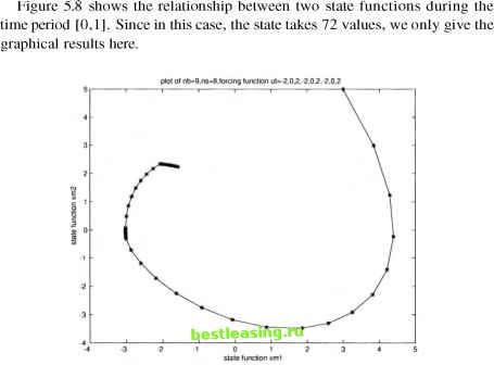

Figure 5.8. Relationship between two state functions during the time period 1,0