mations in this chapter are the essential part of the algorithms in the research, and will be directly applied in Section 2.6.

Consider a financial optimal control model, to minimize an integral:

MINJ= [\x(t)-(t){t)}2dt Jo

(2.1)

subject to:

The time interval [0,1] is divided as follows:

0 = tQ < h < t2 < ... < tj < tj+i < ... < ir i < tr = 1; so there are subintervals:

[to, tl], [h, t2], , [tj-i ,tj], ..., [tr-i,tr].

A scaled time is constructed here to replace the real time in computation; will be used later in the nqq package (differential equation solver). The scaled time rtakes values:

т - 0, h, 2h,jh, (j + l)h,...,(r- l)h, rh = 1

where h = 1/r, thus the time intervals [0, 1] is divided into r equal intervals. The relationship between r and t can be expressed by the following formula:

t = <p(T) = h~l * (tj+i - tj) *(T-h*{j- 1)) + tj (2.4)

where т e [0,1].

Thus the subdivision point t - tj maps to point т = jh. Now the control u(t) takes values:

u(t) = U0,Ul,U2, . ,Uj, . . . ,Ur-l

in successive subintervals:

[0, h], [h, 2h], [2ft, 3ft],..., [jh, (j + l)h], ...,[(r- l)h, 1]

Definex(t) := х(<р(т)).

Then the dynamic equation x(0) - xq, x(t) = u(t) transforms to: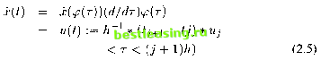

(for jh

The objective function transforms to the sum of integrals: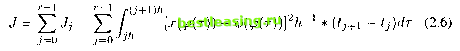

3. Non-linear Time Scale Transformation

In some time-optimal control problems or optimal control problems that are over a long time interval, the large number of subintervals of the time scale will cause computational difficulty. The optimal control functions lead to stable values monotonically when time becomes large. So it would be useful if a suitable non-linear transformation of time scale is practical, (see reference [15, 1998]). With a suitable non-linear time scale, a few subintervals may be enough to get the same accuracy of large subintervals.

Goh and Teo [33, 1987] introduced a change of time scale for a time-optimal control problem while the terminal time T is a variable. Let where

r is the new time variable mapping in [0,1]. t is again written for r, then problem becomes a fixed-time optimal control problem with time interval [0,1] and parameter T. This allows T to be computed accurately without being interpolated between subdivision points.

This makes the original financial optimization problem as the following:

MIN a;(.),u(.) J f{x{t),u{t),t))dt + <b(x(T))

subject to:

x(0) = x0,x(t) = m(x(t),u(t),t)) (0 < t < T)

g(x(t),u(t)) < b(t) {0<t< T) q(x(T)) = 0

Transform into:

MIN x(.)iM(0 jf1 f(x(t),u(t),t))Tdt + Ф(х(1))

subject to:

x(0) = x0,x(t) = rn(x(t),u(t),t))T (0 < t < 1)

g(x(t),u(t)) < b(t) (0 < t < 1) 9(x(l)) = 0

This transformation will be used later in the computational methods 4.1 - 4.5 for the financial model in Chapter 4.

Now consider, an objective function with a discount factor where is positive, thus:

Г e-atf(x(t),u(t))dt Jo

Define time as:

t = -a-llog{\ - рт), where /3 = 1- eaT, т e [0,1]

The objective function becomes:

{P/a) Г f(x(t),u(t))dt Jo