and the differential equation changes from x(t) = m(x(t),u(t),t) to:

For T is fixed and large, the denominator satisfies 1 - (Зт > 1 - j3 > 0. If Г is a variable to be optimized over, then 1 - (3 replaces the variable T, in an interval 0<e<l-/3<.

For example, in a fixed-time optimal control problem, if there is some distinguished time !1 € [0,T], then an additional constraint r(x(T)) = 0 must be satisfied. A transformation of t £ [0, T] to те [0, \] maps T to \, thus to a subdivision point. In particular:

r = h/f (0<t< f), t = 2TY (0 < r < h

At the piecewise-linear transformation is not differentiable, and the

co-state may be discontinuous.

4. A Computer Software Package Used in this Study

The computer package SCOM ([18, 2001]) is a tool to solve step-function optimal control problems on MATLAB 5.2, on a Macintosh computer. It is noted that a program written and compiled in C language will run faster than a MATLAB program for the same computation. However MATLAB is a matrix computation language, so it requires much less programming work in calculating matrix operations on MATLAB than other computer languages, such as C language and Fortran, etc. The program constr is a constrained optimization package in MATLABs Toolbox, based on a SQP (sequential quadratic programming) method. constr will use gradients if supplied; otherwise it will estimate gradients by finite difference. In non-linear programming methods, the SQP method is very successful. The method closely mimics Newtons method for constrained optimization, just as it is done for unconstrained optimization. Using a quasi-Newton updating method , an approximation is made of the Hessian of the Lagrangian function at each major iteration. It is then used to generate a Quadratic Programming sub-problem whose solution is used to form a search direction for a line search procedure. In the research, we build another subroutine to be called as the objective function in constr .

The state functions in this research were solved by the differential equation solver nqq in the SCOM package (see details in Appendix C). When results of the state come out on the grid-points, the objective function J(u) becomes a function of N variables that can also be calculated by

nqq .

When the subroutines for the state functions and objective function are constructed, the MATLAB program constr is then used to obtain the optimal solution of the problem with respect to optimal switching times. In the program, the control и is approximated by a step-function.

5. An Optimal Control Problem When the Control can only Take the Value 0 or 1

From the point of view of control theory, the bang-bang optimal control happens when the systems of the optimal control problems are linear in control. The Nerlove-Arrow model [63, 1962] is an example of a bang-bang control following a singular arc control. Now, introduce a typical bang-bang optimal control problem.

We consider an optimal control problem:

subject to: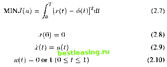

In this case, the statefunction z(.) is assumed piece-wise smooth, and the control u(t) jumps many times between 0 and 1 during the time interval [0, T]. Here, simplify the problem to T = 1. Now use a step-function:

<t) = \ + (-l)fck ) - \\ к = 0,1,2,..., n u(0) = 0 or 1

to approximate the control Here the target function is: Let It.

Observe that if having instead u(t) € [0,1], then u(t) = \ (0 < t < 1) would be optimal, with But if must be either 0 or 1, then

u(t) will jump many times between 0 and 1. Suppose a further restriction is made that, for some given integer n, time interval [0, 1] is divided into n equal subintervals [0,1/n], [1/n, 2/n],..., [j/n, (j+l)/n],..., [(n-l)/n, 1]; takes a constant value (1 or 0) on each subinterval [j/n, (j + l)/n], (j = 0,1,..., n - 1). So if u(t) takes the values in this pattern 1,0, 1, 0, 1,0 on the successive subinterval, then each subintervals contributes l/(12n3) to

as But the optimal value J = 0 is not

reached, unless an infinite number of jumps are allowed.

Now a term К * n is added to the objective function. (2.7) is modified as follows:

MIN F = J(u) + kn= [ [x(t) - <f>{t)]2dt + Kn

Here, K is the cost of changing control and n is the numberoftimeintervals. The objective function of the optimal control problem becomes a cost function. The algorithms in the next section are used for solving these kind of optimal control problems.

6. Approaches to Bang-Bang Optimal Control with a Cost of Changing Control

In this section, the computational methods for solving bang-bang optimal control problems with a cost of switching control are introduced. Simply modifying certain parts of these methods can satisfy a class of similar problems.

Suppose the number N of switching times is fixed by N = nn, say switching times h,t2, . ,tnn. Now consider (2.7) as a function of the switching times, say Then the minimum of this function

is computed, starting from a small value of N. Here the components of the vector are the lengths between each switching

time. The vector um must satisfy the upper and lower bounds 0 and 1, thus 0 < tj-\ < tj < 1, and a constraint Y.i=\ umi = 1 must be satisfied. The vector represents the values of the state func-

tion takes at each switching time. The algorithms are as follows:

Algorithm 2.1 Main Program (see project1 1.m in Appendix A.1)

Step 1. Initialization. Set the maximum number of function evaluations, par, which is the system parameter of the MATLAB constr function, and also another system parameter par(13) = 1 (1 represents the number of the equation constraint in the minimization problem), and a vector of the parameters which are used in the whole subroutines, par = [number of the state components, number of control components, nn= number of total subintervals], arbitrary starting lengths of switching time intervals